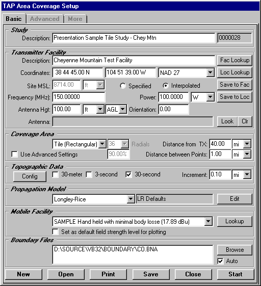
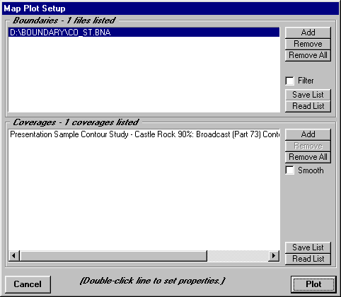
Coverage studies in TAP are set up using the Area Coverage Setup form (opened from the Coverage menu by selecting Area Coverage):

After you have computed a field strength coverage study, TAP will typically provide default values for various parameters for plotting the study. Most of these parameters can be changed to customize the presentation for your needs.

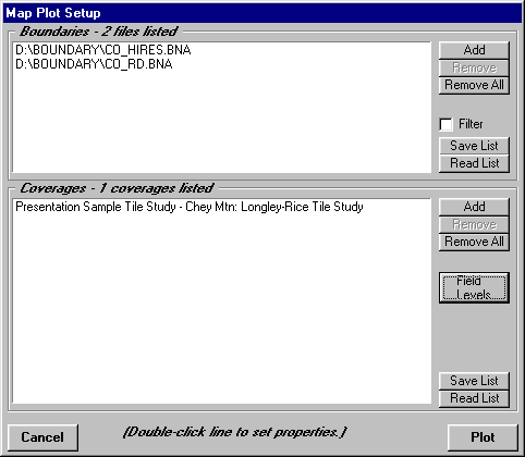
For example, if you compute a tile study, the default values for plotting the study will be displayed on the TAP Map Plot Setup form, including the study coverage and a basic boundary file (the boundary file will normally default to the state where the transmitter site is located if the study is in the U.S.)

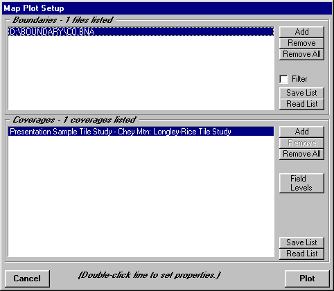
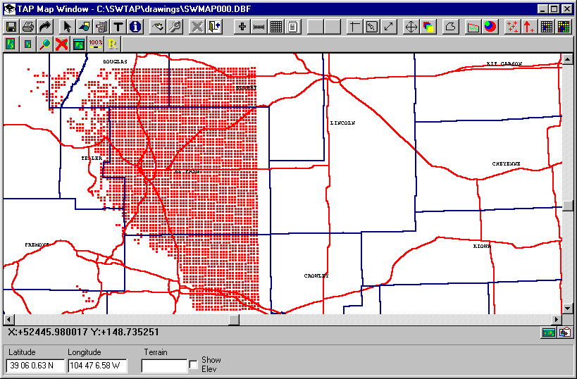
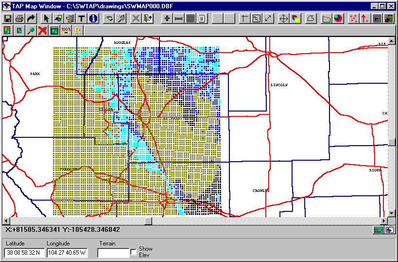
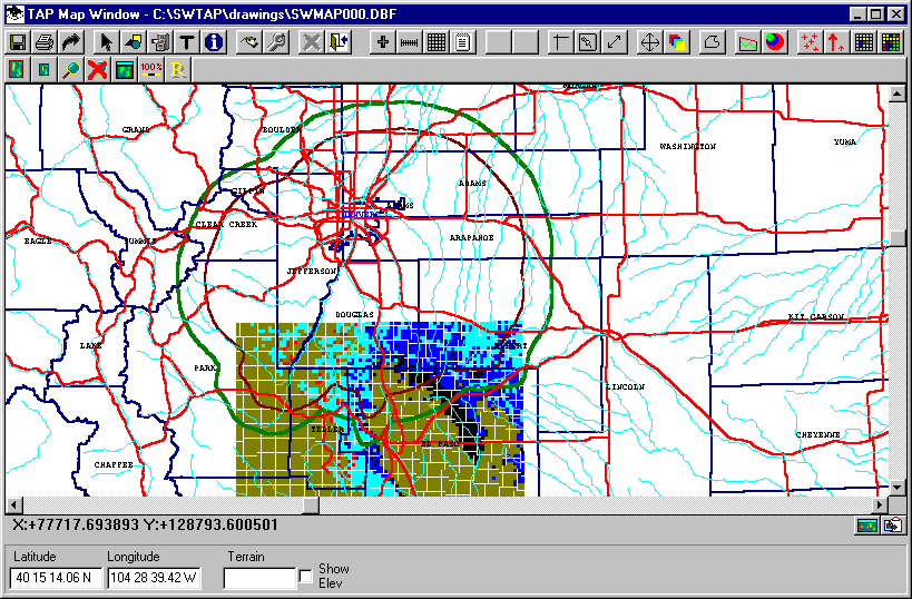
Plotting this study with the default settings will produce a coverage map similar to the one shown below:

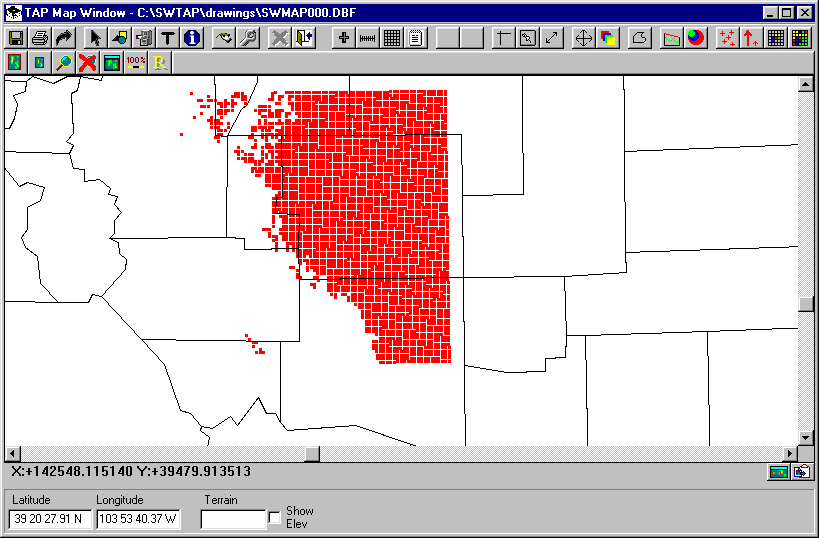
The map shows the basic boundary lines (counties), and a single field strength level in red. The default field level (in dBu) is determined by the Mobile Facility information for required field level used to setup the study. The map indicates where the specified base station (the Fixed Facility) provides coverage at or above that field strength level.

A number of TAP features can be used to enhance the coverage map presentation.

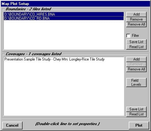
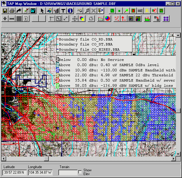
From the Map Plot Setup form, if you have more detailed boundary files, you can remove the original default file (in the case the CO.BNA file for Colorado), and add, for example, the CO_HIRES.BNA file that provides higher resolution boundaries. You can also add other files, such as the CO_RD.BNA file for Colorado roads.

(Note the boundary files contain general information for the borders and main roads. You can also create your own files, or use other files in the Atlas BNA boundary format, or the USGS Digital Line Graph format.)

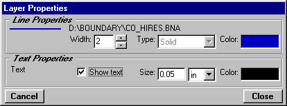
To set the line attributes for the boundary files, you can double-click on each line to set the color and line width for the objects in that file, as well as select the option to display any label information contained in the BNA file:

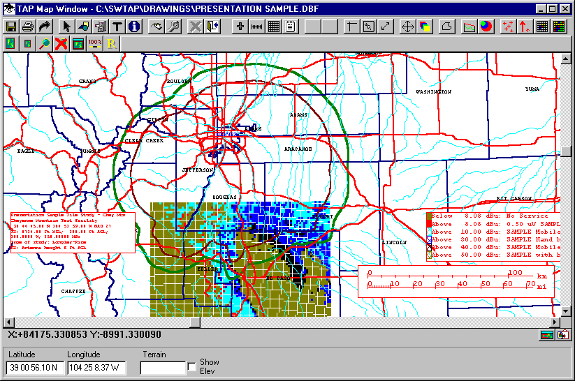
The same coverage plot, with the new boundary files is shown below:

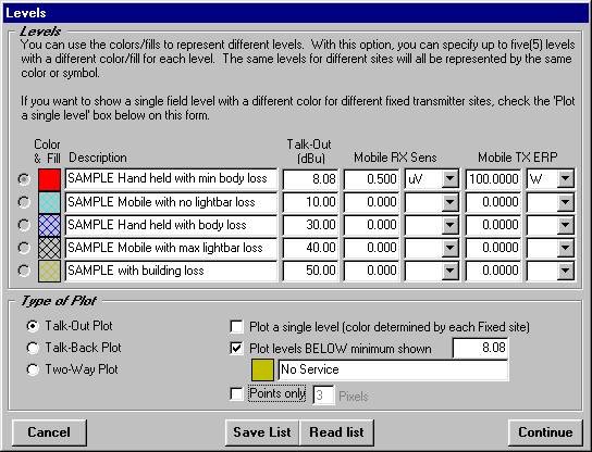
Additional detail can be shown in the coverage information using the Field Levels button on the Map Plot Setup form.

The Levels form enables you to set the field strength values that will be useful to you, such as different levels indicating an adequate signal for different radio and environmental configurations, losses, etc.:

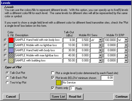
(Note that all field strength levels and other values used in this document are for illustration only. It is important that you determine the appropriate required field levels for your application.)

With these new settings, the coverage map is shown below:

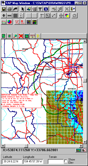
The initial default setting in the Levels form is to draw each field strength point (in a Tile or Radial study) using the "Points only" setting. This forces the program to represent each location as a point of a user specified size, regardless of the zoom factor of the drawing, as shown in the example above.

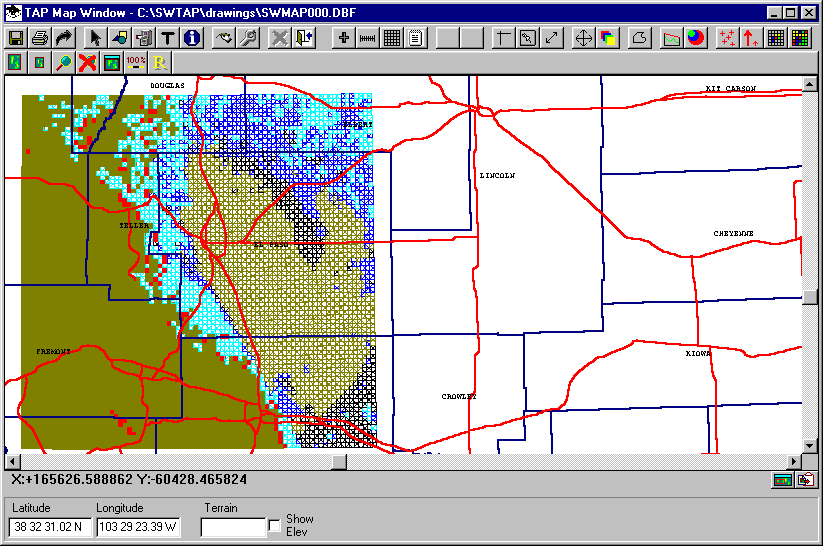
You can remove the Points Only selection on the levels form:

Now the program will draw the area for each computed field strength point to "fill in" the area between the points, and to fill the area with the specified pattern from the levels form, as shown below:

Note that the Points Only option is faster to plot, since drawing pixels is faster than drawing filled boxes.

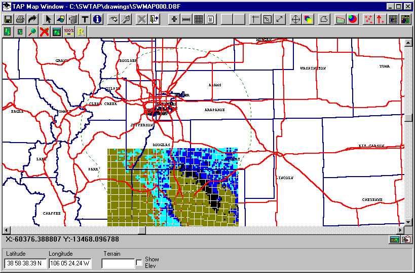
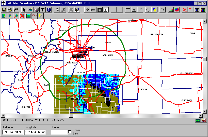
At times it may be useful to show multiple coverages on a single map. This can be included on the Map Plot Setup form using the Add button:

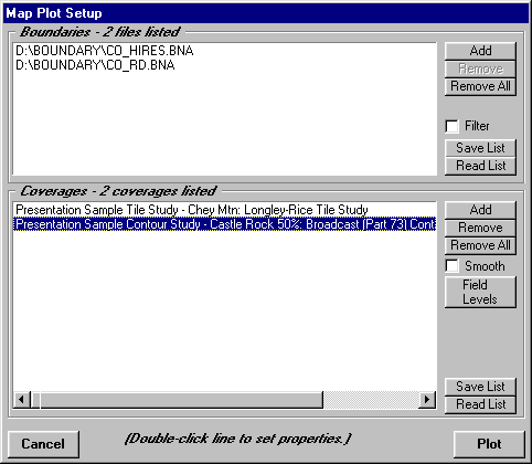
As shown, Tile (and Radial) studies use the values set in the Field Levels button to plot various field values. But Contours (as shown in this example) can be treated like the boundary line entries earlier. You can double-click and set the color and line width for the coverage contour:

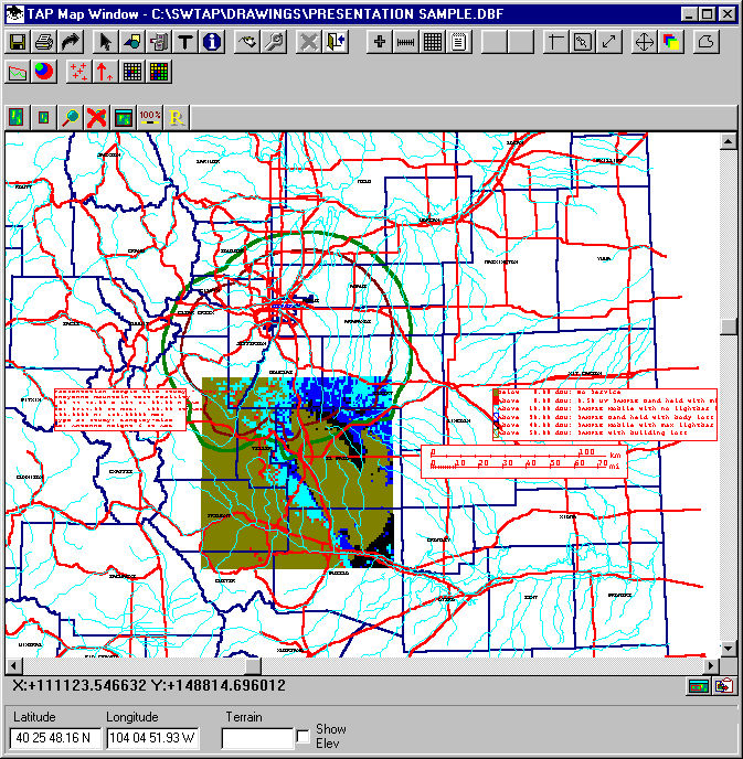
The coverage map will now include both of the specified coverages:

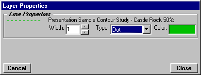
Since the selection of the dotted lines for the coverage contour is difficult to see, you can use the Map Window "Layers" button to change the contour line properties:

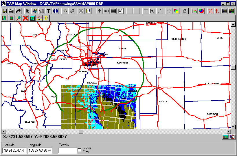
And the change is shown on the map:

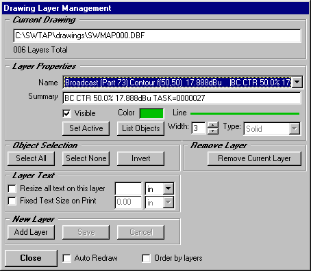
It is often helpful (with complicated drawings) to use the "Order by Layer" feature in the Layers button. For example, the map above shows that the southern part of the coverage contour is partly covered by the tile study values.

This is because the default setting for plotting is optimized for speed, ignoring the order of different layers in the drawing. The Order by Layers option is slightly slower, but usually gives better results:

You can zoom into the Denver area on the drawing and see that there are a number of overlapping labels:

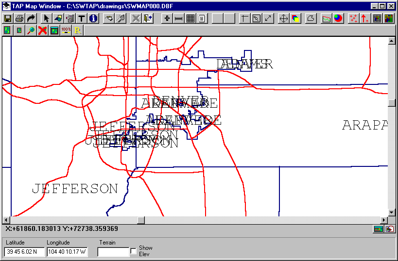
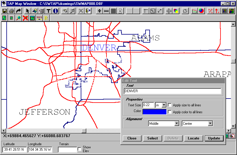
This may occur when labels are repeated for separate parts of the boundary in the BNA file. You can use the Text button on the Map Window tool bar to select and delete the unwanted labels, or to move labels, or to change the color of a particular label:

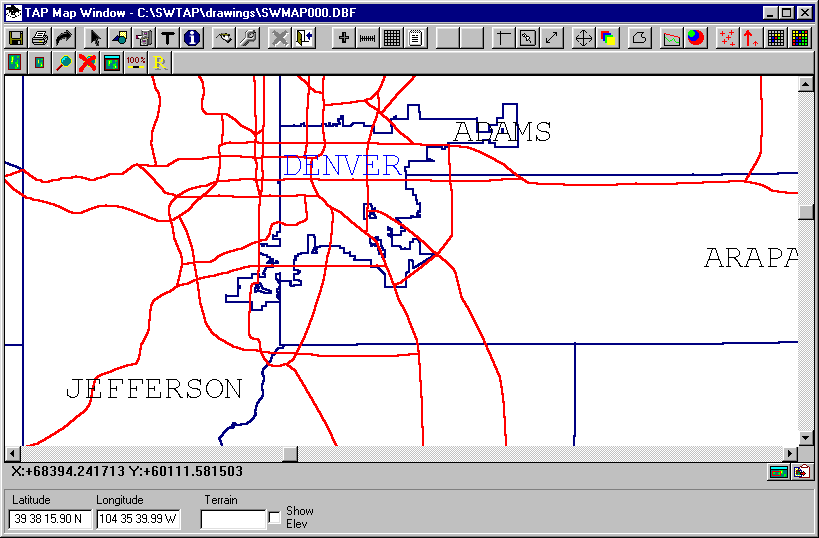
You may also notice some of the lines of the drawing are incomplete after deleting labels or other objects. You can use the Redraw button on the Map Window tool bar to redraw the map:

You can zoom and pan the drawing to display the exact area you want:

You can add boundaries and coverages on the map without going all the way back to the Map Plot Setup form. (However, if you want to change the field strength levels or colors for the plot, you will need to close the plot and set the levels from the Map Plot Setup form.)

Use the Add button on the Map Window tool bar to display a the Map Plot Setup form for adding another contour to the map:

As before you can set the line properties for the new boundary and contour by double-clicking on the line.

The rivers and the new contour will be added to the existing map:

Legends, labels, and a scale can be added to the drawing to show the field levels, coverage parameters, etc.:

When you print the map, you will usually want to use the option to "Print the current graphic window". You can also use the Page Layout function to add information when the map is printed. The Aspect button forces the drawing to change the height and width on the screen to approximate the current printer settings, to help you fit the exact drawing you want onto the printed page.

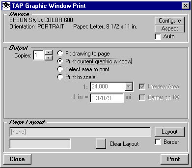
Note, too, when printing, that TAP will attempt to fit the current graphic window to the page. In this example, while the map on the screen is wider than it is high, the default printers setting shown above on the Graphic Window Print form is for Portrait mode. In this configuration, the width of the map will be fit to the width of the page. It would be better to change the printer to Landscape mode to get a better fit of the screen drawing onto the page.

You could also use the Aspect button to force the Map Window on the screen to approximate the page aspect ratio (currently in Portrait mode), but this will dramatically change the window on the screen:

You can always use the mouse to make the Map Window on the screen any aspect ratio you want, just remember that the program will try to adjust to fit the page when printing.

It may be useful to set the window using the Aspect button after first setting the printer to Landscape mode:

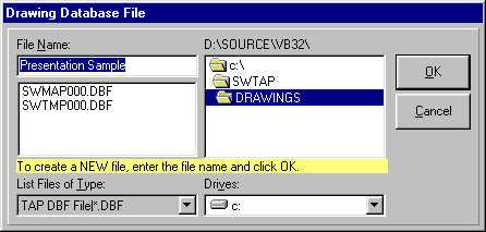
Note that the default graphic database file when you create a map is the file name SWMAP000.DBF. You can save the map to a different file name so it will not be overwritten the next time you draw a map, using the Save button on the Map Window tool bar.

In TAP 4.5 and later, you can include a raster image (such as a .JPG, .BMP, or .TIF file) of a map as a background for the TAP coverage study:

You can use maps you have scanned or obtained from other sources.  The map coordinates can be calibrated to the graphic image the first time you use the image file in TAP.

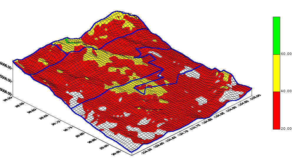
In addition to the features included in TAP for drawing a coverage map, you can also use the Results Data Base file that contains the computed coverage information and import the results into other software.

For example, you can use SURFER to draw the coverage and the topography of the area:

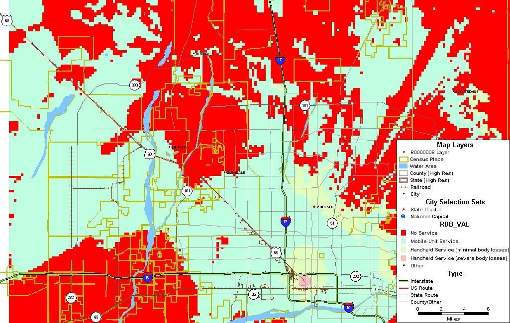
You can use Maptitude or other mapping software to import the coverage results into a detailed map: