HDCoverage™ Introduction
Q: How do I set up a coverage study in TAP using HDCoverage?
A: For TAP 5.0.1056 or later systems with a Maintenance Subscription date of April 30, 2005, or later, area coverage studies can be set up with the HDCoverage software.
HDCoverage is a new user-interface for area coverage functions in TAP. This new interface provides increased flexibility for setting up the base station and mobile unit specifications, and for changing parameters (such as effective earth curvature or surface features) that affect the predicted coverage over the desired area.
Note that all values and settings discussed in this article are for illustration purposes only. It is important for you to determine the particular settings and values applicable to your equipment and application when using TAP.
How does HDCoverage compare with TAP4 Area Coverage Setup?
How do I set up the information for the base station or repeater?
How do I set up the site coordinates and elevation for the site?
How do I set the transmitter frequency and power for the base station?
How do I set up the antenna gain and pattern for the base station?
How do I set up the mobile units to be considered in the study?
How do I set up the antenna height for the mobile units?
How do I determine the signal strength required for the mobile units?
How do I show different signal levels when I plot the study?
How do I define the area I want to include in the study?
How do I decide what kind of study I should run?
How do I set up a study to show a contour for a desired signal level?
How do I set up a study of points along radials from the base station?
How do I set up a study of uniformly spaced points on a grid?
How do I set up the topographic data for the study?
How do I set up the resolution of the elevation data along each path?
How do I set up the method of interpolating elevations from the topographic data files?
How do I set up the study to use 4/3 earth curvature or some other value?
How do I select the propagation model I want to use for the study?
How do I set or change the parameters for the propagation model for the study?
How do I include surface features such as buildings or vegetation in the study calculations?
How do I include USGS Land Use data in the study calculations?
How do I create a new coverage study?
Why do I need to enter a description for the study?
How do I save the study to edit or run later?
How do I open a study I saved earlier?
Why can I not edit some studies? Why does the label say "Locked Task"?
How do I run a study after I have it set up?
A few comparisons and contrasts will help experienced TAP users understand the functions of HDCoverage with reference to the older Area Coverage Setup form.
□ HDCoverage presents the information need to define the coverage study in collapsible panels instead of the tabs and lookup buttons from Area Coverage Setup. While some lookup buttons are still used, the most needed settings and functions are more immediately available when setting up a study using HDCoverage
□ HDCoverage eliminates the distinction used in TAP4 between “basic” and “advanced” studies. The more powerful and yet simplified interface for setting up the coverage area makes this distinction unnecessary.
□ HDCoverage enables you to define a tile area by drawing a rectangle on a map with the mouse. This would be equivalent to the TAP4 “Advanced” Tile study, since the area is not necessarily centered on the fixed facility site.
□ HDCoverage introduces the “Target” study, in addition to the Contour, Radial, and Tile studies supported in TAP4. The Target study is similar to the Advanced Radial study using the “End points only” option. You can define target point locations and the field strength will be computed at those locations, but not along the entire path from the fixed facility to the point (as would be the case with a Radial study). You can define target points by entering coordinates (and an optional description) manually, or you can click points on the map, or you can read the point locations from a Shapefile. Importing .BNA files into HDCoverage is not supported (as it was in TAP 4 Advanced studies). However, TAP4 still includes a utility for converting .BNA files to the Shapefile format.
□ HDCoverage allows you to define a Tile study using a polygon shape (such as a county boundary). The boundaries are read from Shapefiles. As mentioned above, the previously supported .BNA files can be converted to Shapefiles in TAP4.
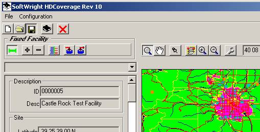
HDCoverage presents almost all the pertinent information for an area coverage study on a single form.
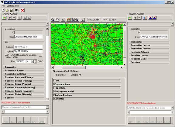
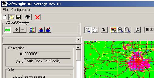
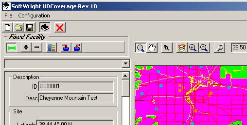
When HDCoverage is launched, the area form is displayed:
This form displays the Fixed Facility Database Interface (on the left side) for the base station, repeater, etc., and the Mobile Facility Database Interface (on the right side). The other parameters needed for the study (area of coverage, propagation model, etc.) are in the center of the form at the bottom. A map is provided to facilitate the definition of the coverage area to be computed.
The Fixed Facility Database enables you to create records representing existing, proposed, or hypothetical base stations, repeaters, or other types of antenna sites. You can create records representing facilities that actually exist, as well as other “what if” facilities for various studies.
The use of the Fixed Facility Database is described in more detail in the Fixed Facility Database Interface article. In general, you can use the scroll bar near the bottom to scroll through the existing records, or you can use the pulldown list (just above the scroll bar) to view a list of the records in the database to select the facility you want to use.
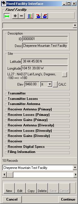
You can also use the “New” button (at the bottom of the interface) to create a new record, or the “Copy” button to copy the current record so you can edit certain parameters.
In addition, you can use the “Disconnect” button (at the top of the interface) to disengage the interface from the database. This enables you to enter and edit values without affecting the records in the database.
The Fixed Facility database includes a large number of data elements, down to details such as the amount of loss to be included for connectors in the transmission line path, etc. While it is useful to include all of this information, only certain values (or “fields”) are absolutely required for a coverage study using HDCoverage.
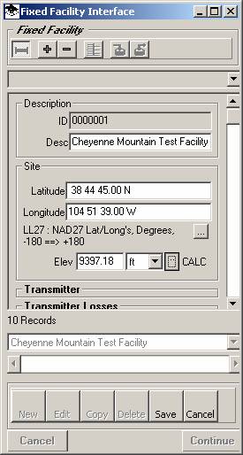
You must enter the site coordinates and an elevation for the site.
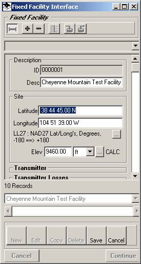
The coordinates can be entered in any of the dozens of coordinate systems supported, such as latitude and longitude, state plane, UTM, etc., by clicking the button to the right of the coordinate system description:
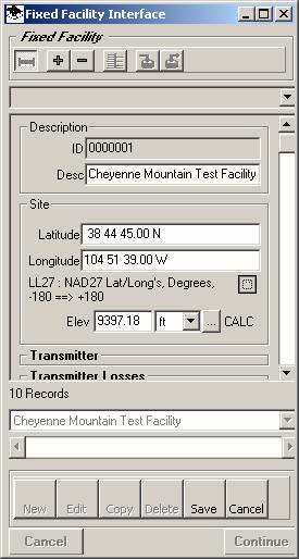
You can enter a value for the site elevation manually (from a map, station license, survey, etc.), or you can click the button to the right of the elevation to get the elevation value from the available topographic data.
You must enter the transmitter frequency:
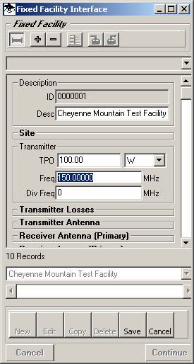
The Transmitter Power Output (TPO) can be used to compute the Effective Radiated Power (described below). This enables you to enter the TPO value, along with the antenna gain and system losses (transmission line, component insertion losses, connectors, etc.) to compute the ERP. The ERP value can also be entered directly (as described below), since that is the value actually used in the field strength calculations in the area coverage sturdy. If the ERP value is entered directly it is not necessary to enter the TPO and various gain and loss values.
The Diversity Frequency value – “Div Freq” – is only used for microwave link budget calculations involving frequency diversity.
You must enter the transmitter antenna height and the Effective Radiated Power (ERP).
The transmitter antenna height is the height of the antenna center of radiation:
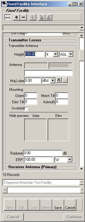
You can use the Antenna Lookup button (to the right of the Major Lobe gain value in the Transmitter Antenna section) to select an antenna pattern from one of the TAP Antenna Libraries:
When you click the Antenna Lookup button, you will first be prompted to select the library you want to use:
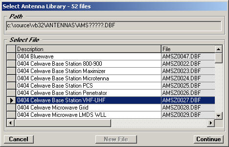
Select the library file you want to use by clicking the selection button to the left of the row to highlight the row. The Antenna Library files can be one of the sample files supplied with TAP, or an antenna library you created by importing pattern information.
When you have selected the library file you want, click the Continue button. The Antenna Editor will be displayed:
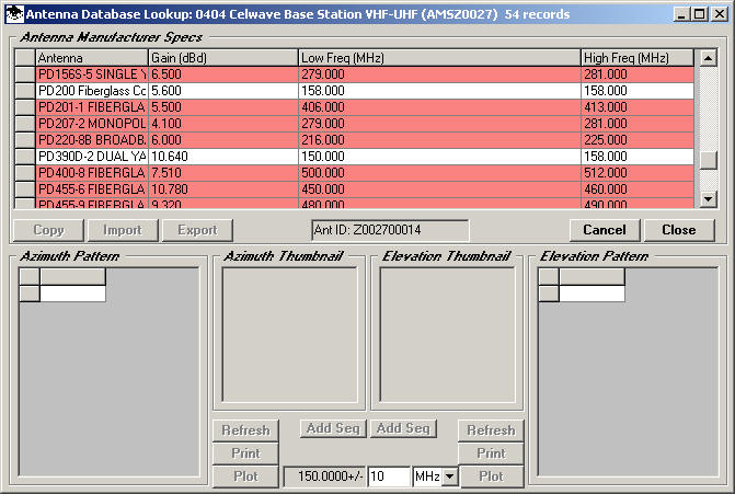
The frequency from the Fixed Facility record is displayed near the bottom center of the form. You can specify a range of frequencies, such as +/- 10MHz to find patterns in the library with frequencies near your operating frequency. Naturally, whenever possible, you should obtain measured pattern information from the manufacturer for the exact antenna and exact frequency of your facility. The frequency range option is provided to find antennas that may have similar gain and pattern characteristics if the library does not contain a pattern measured on your frequency.
The antenna records will be displayed with a white background if the frequency range in the library for the antenna is within the range you specified. Antennas with frequencies outside your specified range are displayed with a light red background. (Some library files do not include frequency information, and values of zero are displayed.)
Select the antenna record you want by clicking on the selection button to the left of the row to highlight the row:
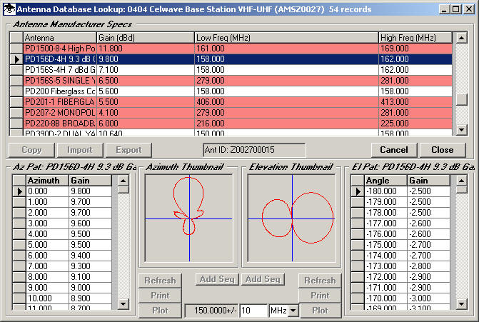
A small "thumbnail" of the azimuth and vertical patterns associated with that antenna are displayed, as well as gain information on horizontal azimuths and vertical angles. (This information cannot be edited in Lookup mode. If you want to edit or add antennas manually, or import antenna files, use the Antenna Editor function from the main menu.)
Click the "Close" button to return the selected antenna information to the Fixed Facility record.
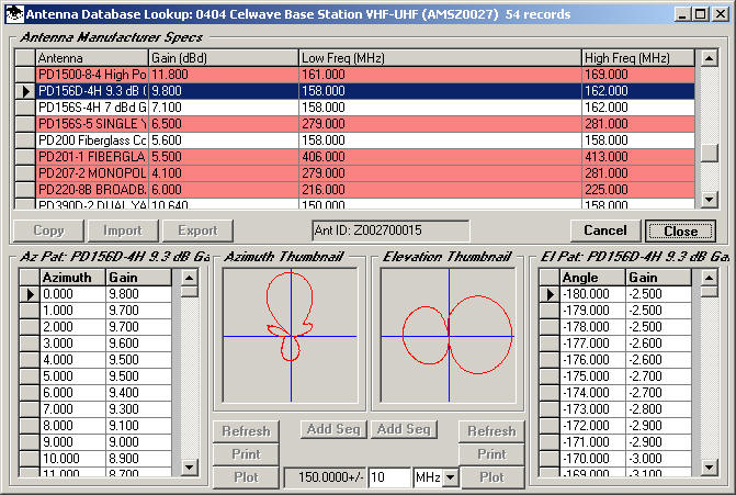
(To cancel the operation and close the form without returning antenna information to the Fixed Facility record, click the "Cancel" button.)
When the Antenna Lookup form is closed, the antenna information is returned to the Fixed Facility record:
The antenna pattern thumbnails are displayed in the Fixed Facility Record.
The "Mounting" parameters can be used to specify the azimuth orientation of the pattern and the tilt of the elevation pattern. For example, if your application requires the major lobe in the horizontal (azimuth) plane be on a bearing of 45° True, enter a value of 45 for the antenna Orientation:
To add tilt to the elevation pattern, enter the value as either Electrical or Mechanical tilt:
Note that the thumbnail patterns show the approximate pattern orientation and tilt values.
The Electrical Tilt function adjusts the library pattern by the specified value. If you expect to use an antenna with electrical tilt provided by the manufacturer, you should obtain the measured pattern information for the antenna with beam tilt from the manufacturer. If the library pattern already has the electrical tilt included, you should not enter a tilt value for the Fixed Facility record.
The program handles electrical and mechanical tilt differently. For electrical tilt, the program assumes that the pattern is tilted the same amount on all azimuths. For mechanical tilt, enter the azimuth of the direction of the tilt (usually, but not necessarily, the azimuth of the major lobe). The effective tilt on a given azimuth is a cosine function of the tilt on that azimuth.
The ERP (Effective Radiated Power) is the power output from the transmitter (TPO) plus the antenna major lobe gain, minus all the losses from connectors, transmission line, radome, etc. If you enter the TPO, antenna gain, and the loss values, the ERP will be computed automatically.
Note that if you change a related value (the TPO, gain, or loss values) the ERP will be automatically re-computed:
Since you can enter the ERP value directly it is possible to enter approximate values or estimates or “what if” power levels for a preliminary study. You can later go back and do a more precise calculation by entering the TPO and other values to get the exact ERP to be used.
Note that the “Receiver” sections in the Fixed Facility Database Interface are for the receiver at the base station, not the mobile receiver. The mobile facility information for the handheld, pager, vehicle radio, etc., to be used for the study are entered using the Mobile Facility Database Interface described below.
The Receiver information for the Fixed Facility is needed for talkback studies of the system.
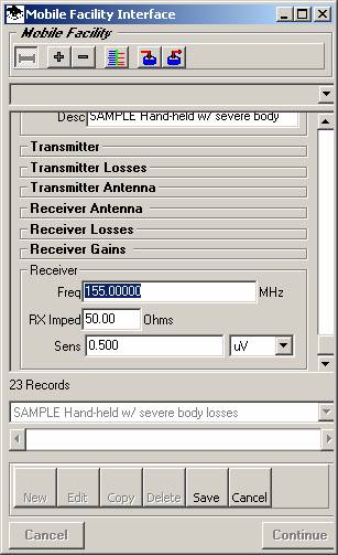
The Mobile Facility Database enables you to create records representing different mobile unit configurations you want to use in your coverage studies. The Fixed Facility Database (discussed above) is intended to have one (or more) records for each facility. The Mobile Facility Database is intended to contain one record for each type of radio, or for each set of circumstances to be considered.
For example, you might have an organization that uses 100 portable units, but there are only two different models, with different characteristics (antenna gain, etc.). If you wanted to run coverage studies to see how the use of those two models of radio would affect your coverage, and you wanted to consider them under three different conditions (ideal, good, and poor), you could set up six Mobile Facility records. For each radio model you would have records that included no environmental losses, minimal losses, and severe losses. (For a discussion of setting required field strength values and the use of loss values, such as body loss or building losses, see the Required Field Value article.)
Like the Fixed Facility Interface, you can use the scroll bar near the bottom to scroll through the existing records, or you can use the pulldown list (just above the scroll bar) to view a list of the records in the database to select the facility you want to use.
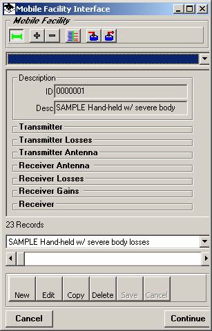
You can also use the “New” button (at the bottom of the interface) to create a new record, or the “Copy” button to copy the current record so you can edit certain parameters.
In addition, you can use the “Disconnect” button (at the top of the interface) to disengage the interface from the database. This enables you to enter and edit values without affecting the records in the database.
The Mobile Facility database includes a large number of data elements, down to details such as the amount of loss to be included for connectors in the transmission line path, etc. While it is useful to include all of this information, only certain values (or “fields”) are absolutely required for a coverage study using HDCoverage.
You must enter the antenna height for the mobile unit.
The same antenna is assumed to be used for both the receive and transmit functions of the mobile unit. You must enter the antenna center of radiation height:
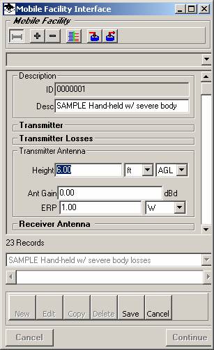
The antenna height is used for computing the path geometry between the base station and each mobile location defined for the study (for line of sight, path obstructions, etc.). You might also want to create separate records for the same radio used at different heights, for example, 3ft AGL for a belt holster, and 6ft AGL when held to the mouth.
The antenna elevation reference (AGL or MSL) affects how the mobile is treated in the coverage study. Typically land mobile units are specified as AGL (the antenna height above ground level). With this setting, the mobile antenna follows the ground elevations, always remaining at the desired height relative to the ground level.
The MSL reference is used for ground-to-air studies. When the mobile antenna elevation is set, for example, to 30,000ft MSL, the antenna elevation is independent of the terrain elevation at that location, representing an aircraft in level flight over the variable terrain. (Ground-to-air studies in TAP should only be performed using the Bullington or Shadow modules, since other propagation models are limited on the nominal antenna height above ground. For more information, see the Propagation Comparison article.
If you are computing a Contour study (see the Coverage Area discussion below), you must enter the Required Field value to be used for the contour to compute:
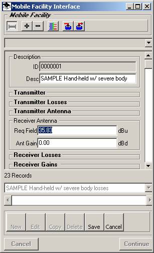
The Required Field value can also be computed by entering other parameters, such as the manufacturer’s specified receiver input level, antenna and preamp gains, losses for transmission line, connectors, etc., as well as environmental losses such as body loss, vehicle loss, and building loss. . (For a discussion of setting required field strength values and the use of loss values, such as body loss or building losses, see the Required Field Value article.)
If you are computing a Tile, Radial, or Target study, you can change the desired value(s) of required field which you want to plot when you draw the coverage map. The setting for the Required Field value in the Mobile Facility Interface that is used for the study does not restrict you to only plotting that level for the Tile, Radial, or Target study. Typically, that plot is the point where you will use the required field values from different Mobile Facility records, such as red for all the points that meet the requirement with severe body losses (one required field value) and blue for all the points that meet the requirement for minimal body losses (a different, lower required field value).
The field strength plotting and setting the desired field levels is discussed in the RF Field Strength Levels article.
If the frequency of the mobile receiver is not set, or does not match the Fixed Facility transmit frequency, it is ignored and the Fixed Facility transmit frequency is used.
The Mobile receiver frequency is important when you are computing (rather than entering manually) the required field value, or computing transmission line loss, or other equipment parameters that are frequency-dependent.
HDCoverage supports four methods for defining a coverage area study:
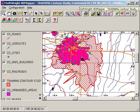
□ Contour studies compute a single closed polygon defining a signal level for a user-specified percentage coverage. Contour studies are computed from calculations along radials from the fixed facility. On each radial, a distance is defined where the defined signal level is met or exceeded at the desired percent of the points on that radial. For example, if you compute the 39dBu contour for 95% of the points, the contour that is computed and plotted will be a polygon that connects all the radials. The 39dBu level would be met or exceeded at 95% of the points computed inside the contour. That means that 5% of the points would be below that level. The exact location or field strength of the deficient points are not shown by the contour calculation or plot.
□ Radial studies compute the field strength at points on radials from the fixed facility location at uniformly spaced locations along the radial, out to a specified distance. The radial azimuths, length, and point increment are all user-defined. You can specify radial azimuths over a desired aperture, or equally spaced radials all around the fixed facility, or you can enter individual radials by azimuth, length, and increment. The radial study can be any combination of these types of radials. For example, you may want to compute the radial study out 30 miles all around your fixed facility on 5 degree azimuths (0 to 355), with points computed every half mile. But your main area of interest might be to the southeast, so you could specify radial on one-degree azimuths with points computed every tenth of a mile for azimuths 120 to 140 to cover the area. The HDCoverage setup gives you significant flexibility in setting up the study you want.
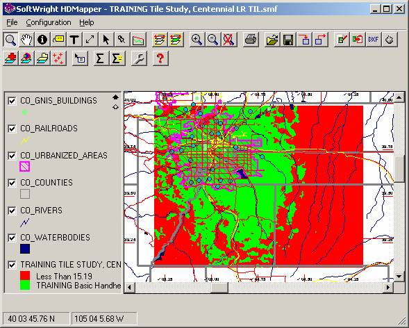
□ Tile studies compute the field strength at points on a uniform rectangular grid. You can define the area of that rectangular grid by specifying the north, south, east, and west boundaries, or you can specify a range out from the fixed facility, or you can click an area on the HDCoverage map to define the limits of the area. If you want to compute the points on the grid intersections only within a particular boundary, such as your county, you can use a Shapefile of that county boundary to limit the calculation only to points within that polygon.
□ Target studies compute the field strength at specified points. Unlike a Radial study, the field strength is only computed at the end point, not at all the points along the path between the fixed facility and the point. Unlike a Tile study, the points are not required to be on a uniform grid but can be arbitrarily located. You can define target points by entering coordinates (and an optional description) manually, or you can click points on the map, or you can read the point locations from a Shapefile.
The type of area you select depends on the type of results you are looking for.
Contour studies are the most simple presentation, especially for a non-technical audience. However, it is important to understand that there will be un-served locations within the contour (the deficient 5% in the example above) and there is no way (using only the contour) to know where the points will be. It is equally important to understand that there will usually be locations with good service outside of the contour. If there are enough locations along a radial with poor signal strength (say, due to a hill close to the fixed facility in the direction of that radial), the percentage value required may cause the contour to be pulled in close to the fixed facility. But if the terrain rises farther out on the same radial, the signal may actually improve for more distant points that rise out of the shadow of that hill. For a further discussion of how contour locations are computed, see the Contour Interpolation Calculation article.
Radial studies will usually be faster to compute than Tile studies. For a radial study consisting of 360 radials out 10 miles, computing the field strength every tenth of a mile, the program will compute 36,000 field strength values. But since many of the points are on the same radial, involving the same topography, only 360 paths are required. The program reads all the data on the zero-degree azimuth and uses that data to compute all 100 points on that radial, and so on. A Tile study out 10 miles on a tenth-mile grid would compute about 40,000 points (a 200x200 grid). But since the grid intersections do not align on the same azimuths (like a Radial study), the program must retrieve the topo elevation values for 40,000 independent paths. While TAP includes optimization to make this process as efficient as possible, Tile studies will generally take longer than comparable Radial studies. One implication of this fact would be that if you are running studies as a preliminary comparison of five different sites to determine the best likely location for a new repeater, using radial studies will give you the quickest results for comparison.
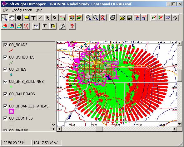
Tile studies provide more uniform detail than Radial studies. Radial studies have the disadvantage that the radials diverge, and at significant distances the “gap” between the ends of adjacent radials can grow unacceptably large. Even though the assumption would be that the unknown field strength between two radials is similar to the adjacent values where radials were computed, it still remains unknown. For example, for a Radial study out 20 miles with azimuths every 5 degrees (72 radials), the distance between the ends of adjacent radials will be 1.75miles. The Tile study avoids this problem by using a uniform grid spacing over the entire area. Trends and variations in field strength levels are usually easier to see in the uniform tile presentation, and the detail is the same over the entire study, avoiding the “spokes of a wheel” look of a radial study. To continue the example above, after using faster Radial studies to pick the best repeater site, you might want to use a Tile study for the file report showing the coverage from your new installation. Tile studies also have the flexibility of being anywhere in the area around the fixed facility, while Radial studies are, by definition, centered on the site.
Target studies enable you to focus on the points of highest interest. For example, in trying to determine the best possible repeater site in our hypothetical situation, you might be able to define one or two or several dozen critical points (highway intersections, business districts, etc.) where you are most concerned about improving coverage. Using a Target study to compute the field strength values at each of those decisive locations might help you eliminate one or more of the potential repeater sites in a very short time. Target studies are useful for point-to-multipoint systems, such as from a control center to pumping stations or well heads. But the field calculations are performed only at the specified locations and do not show trends or sudden changes in the field strength predicted. For example, if a highway intersection is a critical location for the proposed repeater, it would be wise to include a point or two along the highways on either side of the intersection to be sure the signal is available in the vicinity of the intersection.
The type of coverage area, and the specifications for the area, are defined in the Coverage Area Settings section in the bottom center of the HDCoverage form:

This section includes several parts of the coverage study parameters:
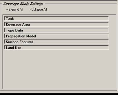
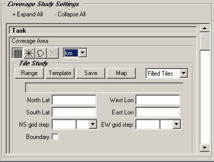
You can expand and collapse sections by clicking on the title. For example, if you click on Coverage Area, that section of the form expands:
The buttons across the top of the Coverage Area section enable you to define the type of coverage area you want.
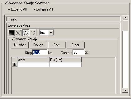
To create a Contour study, click the button showing a simple polygon contour:
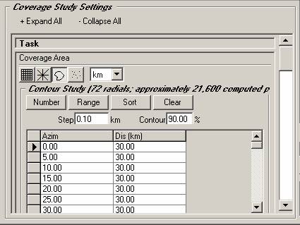
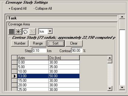
The form will change to the Contour settings:
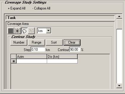

The step along the radials is important for Contour studies computed with analytical propagation models such as Bullington, Longley-Rice, or Okumura. The Step Distance determines the resolution of the contour location. In this example, the contour will be located to the nearest 0.1kilometer along each radial. For calculations with statistical propagation models such as FCC Broadcast or Carey, this value is not used, since the calculation is based only on the height above average terrain (HAAT) using the topographic data parameters set in the Topo Data section as described below.
Set the step value on the form:

You can define the azimuths on which you want to compute the contour. For example, suppose you want to compute 72 equally spaced radials. Click the “Number” button:
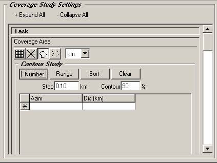

You will be prompted to enter the number of radials to create:
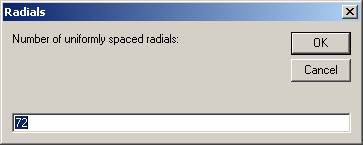
You will be prompted for the range of the radials from the fixed facility:
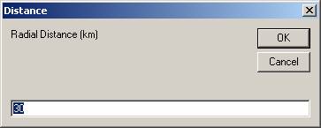
When the number and length for the radials have been entered, the program creates the radials for the contour calculation:

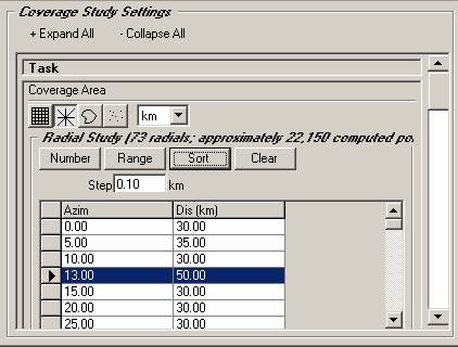
You can edit individual values on each radial:
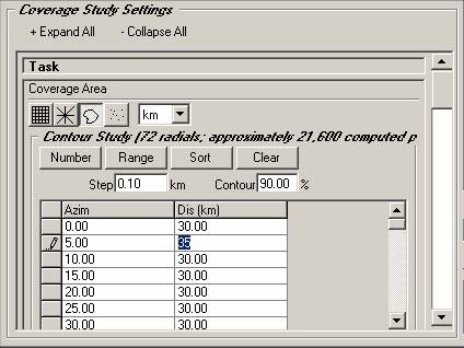

Note the pencil icon at the left end of the row indicating that the value is being edited. You can undo the edit as long as the pencil is displayed by clicking the Esc key on your keyboard and the original value will be displayed.
You can delete a row by selecting it by clicking on the selection button to the left of the row and clicking the Delete key on your keyboard.
You can add individual radials by scrolling to the end of the list to the row with the asterisk (“*”) in the selection button.
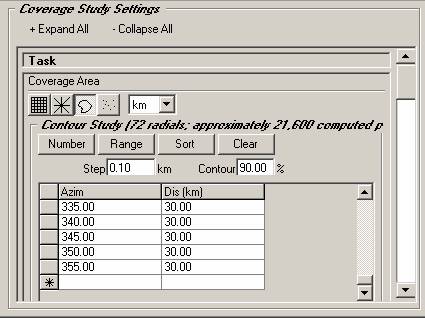

When you start typing on that line, a new azimuth record is created:

You can fill in the desired values in each column:
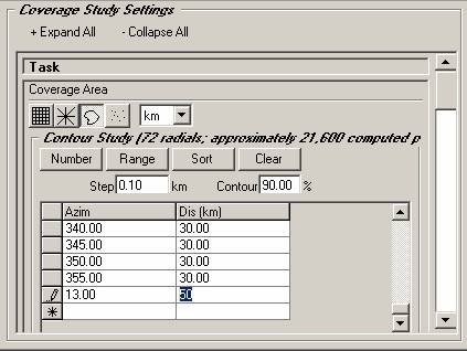
Click another line to move off of the new line so the pencil icon disappears. This is necessary to be sure the new added azimuth is saved.
Click the Sort button if you want to see the radials displayed in order by the azimuths. (The program automatically sorts the radials when the coverage study “Task” is saved, as described below.)

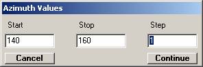
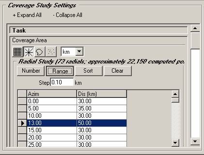
You can also define a range or aperture of azimuths. For example, suppose you are particularly interested in the area to the southeast of the Fixed Facility and you want to compute the contour every 1 degree (instead of every 5 degrees) over that range. Click the Range button:


You will be prompted for the range and increment of the azimuth values:
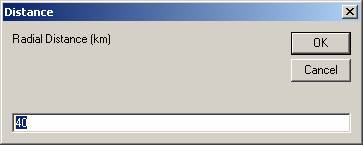
You will be prompted for the length of the radials to compute for the contour:
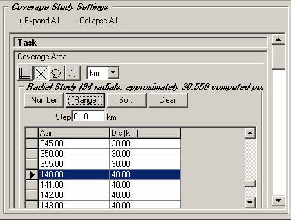
When these values have been entered, the new azimuths will be added at the end of the list:
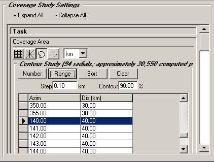

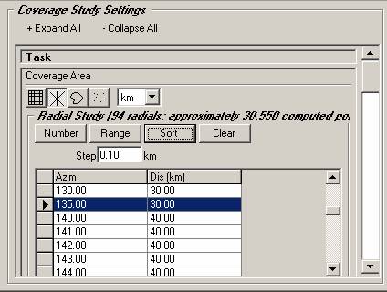
You sort the azimuths to put them in the correct order. In this example, there will be some duplication of azimuths. The original 72 azimuths created rows for azimuths 140, 145, etc., which were 30 kilometers long with a step value of 0.1 kilometer. The range of radials from 140 to 160 also created entries on some of the same azimuths (140, 145, etc.) but with different length and step settings (40 kilometers, 0.05 kilometers).
The program resolves this ambiguity of duplicate azimuth values by always using the longer distance and the smaller step value. This change is applied when you Sort the list:
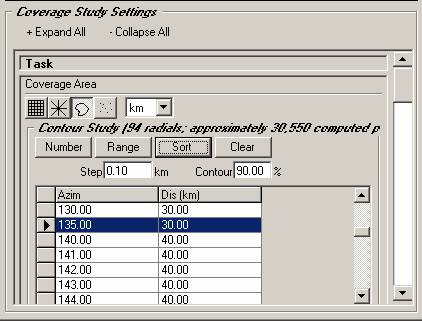

The contour setting also requires a value for the percentage value to be used in locating the contour on each radial. For example, if you set the value to 90%, the contour will be located on each radial at the location where at least 90% of the computed field strength points on that radial meet or exceed the Required Field value specified in the Mobile Facility Interface.
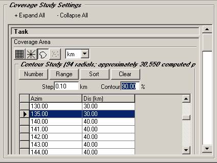

For additional information about the contour calculation using the percentage value, see the Contour Interpolation Calculation article.
Note that this percentage value is used for analytical propagation models (Bullington, Longley-Rice, Okumura, etc. Statistical models (FCC Broadcast, Carey, Specialized Mobile Radio) include a percentage value in the propagation model. This value is describe in the Propagation Model section below.
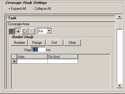
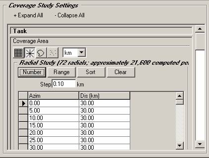
To create a Radial study, click the button showing the radials:

The step along the radials is important for radial studies computed with analytical propagation models such as Bullington, Longley-Rice, or Okumura. The Step Distance determines the resolution of the computed point locations along the radial.
Set the step value on the form:
You can define the azimuths on which you want to compute the field strength values. For example, suppose you want to compute 72 equally spaced radials. Click the “Number” button:
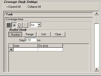

You will be prompted to enter the number of radials to create:
You will be prompted for the range of the radials from the fixed facility:
When the number, length and step for the radials have been entered, the program creates the radials for the calculation:

You can edit individual values on each radial:
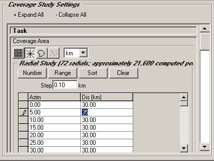

Note the pencil icon at the left end of the row indicating that the value is being edited. You can undo the edit as long as the pencil is displayed by clicking the Esc key on your keyboard and the original value will be displayed.
You can delete a row by selecting it by clicking on the selection button to the left of the row and clicking the Delete key on your keyboard.
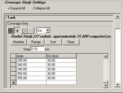
You can add individual radials by scrolling to the end of the list to the row with the asterisk (“*”) in the selection button.
When you start typing on that line, a new azimuth record is created:
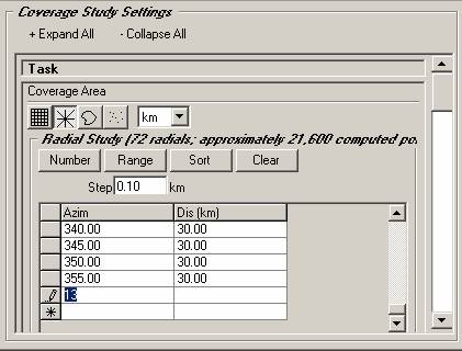

You can fill in the desired values in each column:


Click another line to move off of the new line so the pencil icon disappears. This is necessary to be sure the new added azimuth is saved.
Click the Sort button if you want to see the radials displayed in order by the azimuths. (The program automatically sorts the radials when the coverage study “Task” is saved, as described below.)
You can also define a range or aperture of azimuths. For example, suppose you are particularly interested in the area to the southeast of the Fixed Facility and you want to compute the contour every 1 degree (instead of every 5 degrees) over that range. Click the Range button:
You will be prompted for the range and increment of the azimuth values:
You will be prompted for the length of the radials to compute for the contour:
When these values have been entered, the new azimuths will be added at the end of the list:
You sort the azimuths to put them in the correct order. In this example, there will be some duplication of azimuths. The original 72 azimuths created rows for azimuths 140, 145, etc., which were 30 kilometers long with a step value of 0.1 kilometer. The range of radials from 140 to 160 also created entries on some of the same azimuths (140, 145, etc.) but with different length and step settings (40 kilometers, 0.05 kilometers).
The program resolves this ambiguity of duplicate azimuth values by always using the longer distance and the smaller step value. This change is applied when you Sort the list:

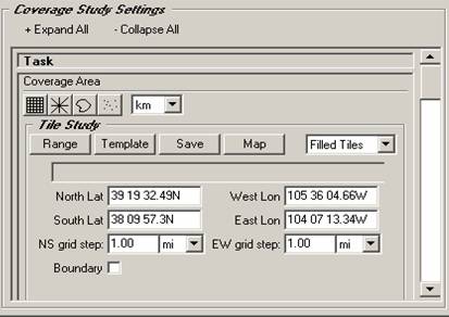
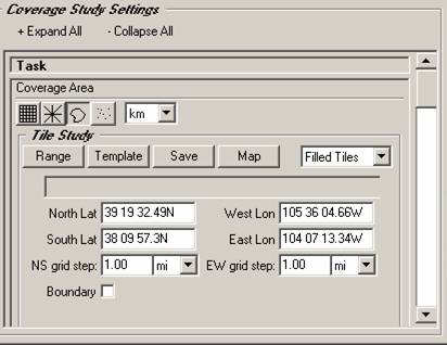
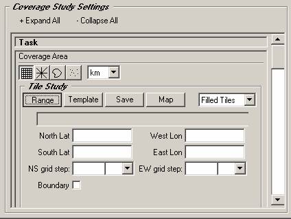
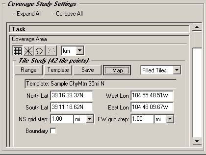
To create a Tile study, click the button showing the uniform grid of points:

The form will change to the Tile settings.
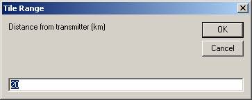
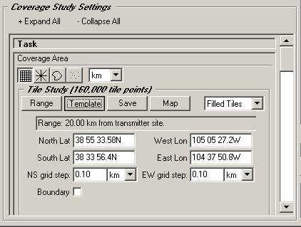
You can define the Tile area as a range measured from the Fixed Facility site. For example, suppose you want to compute the area for a range of 20km from the site (a 40 x 40km square). Click the Range button:
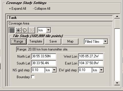
You will be prompted for the range from the site:
When you enter the range, the latitude and longitude limits of the area will be computed and displayed:

Another way to set the boundaries of a tile area study is to use the TAP Area Template database. This is a database of tile area limits that can be used to define exactly the same tile area for several different studies. For example, if you want to compare the coverage of an area of interest from two (or more) different repeater sites you can use the Area Template to ensure that you compute the coverage for exactly the same area. The Area Templates are also used for TAP Aggregate Coverage studies, where signal levels from multiple sites can be compared or combined (such as Best Server studies or Simulcast studies.
To use the Area Template, click the Template button:
The Area Template form will be displayed.
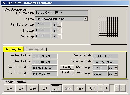
Select the template you want to use (or create one with the New button). When you click Close, the area limits will be returned to HDCoverage and displayed on the form:
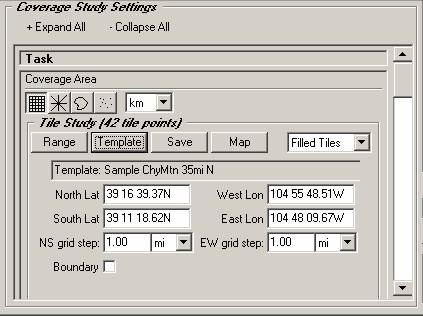

If you define a tile area you can also use the Save button to write that area as a new Template in the database for future use.
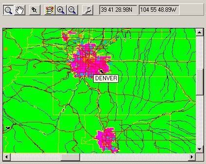
With HDCoverage, you can also define the tile area graphically on the map.
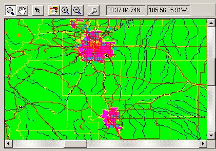
Be sure the magnifying glass button is pressed, then click and drag a rectangle on the map to zoom into the area of interest:
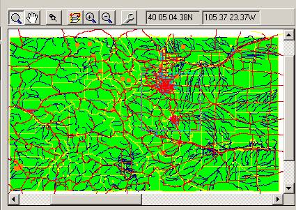

The map will zoom to the area defined by the mouse rectangle you drew:

You can locate the Fixed Facility site on the map by clicking the Pin button:
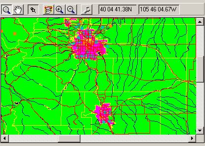

The location of the site will be displayed on the map (note the green triangle near the bottom center of the illustration). Clicking the Pin button will cause the site to flash, making it easier to locate.
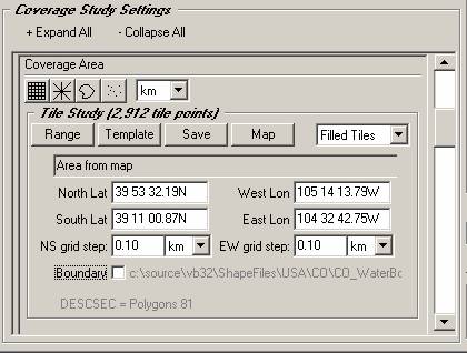
When you are ready to define the tile area on the map, click the Map button:

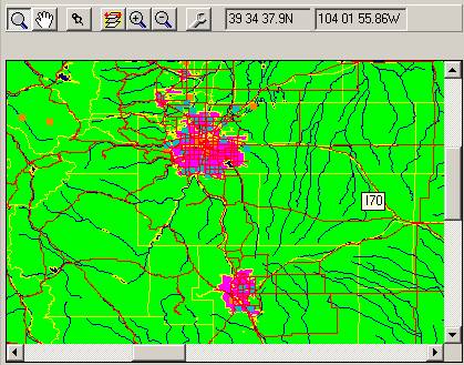
You will be prompted to draw the desired tile area on the map with the mouse. Click one corner and drag the rectangle to the opposite corner:
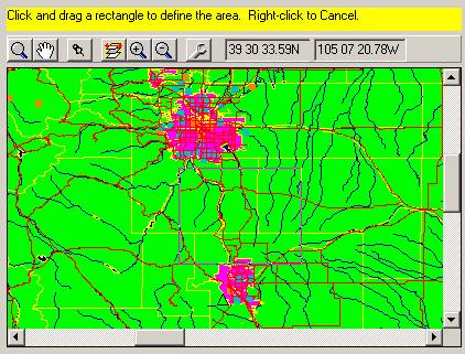
When you release the mouse, the coordinate limits of the area will be displayed:
Another option for setting the area for the Tile study uses a Shapefile to define the boundary. With this option, the points are still computed on the rectangular grid points, but the area is limited to points inside of the selected boundary.
The map consists of a separate layer for each shapefile used in the map. You can select the active layer to use when you are selecting a boundary object to use for the Tile study.
To select or change the active layer, right click on the map. The “Select Active Layer” dialog box is displayed:
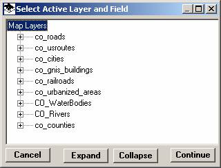
This dialog box displays the current layers on the map, in the order they appear. The top layer in the list is also the top layer on the map.
Each layer may contain one or more “fields” or data values associated with the objects on that layer, such as county names, highway numbers, population information, etc.
If you click the “+” symbol for a layer you can view the fields for that layer:
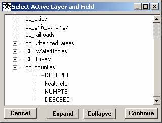
(Remember, the actual layer and field names will depend on the shapefiles used in your map.)
To select the active layer and field, click the item on the tree list:
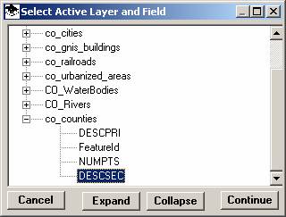
Click the Continue button to make the selected layer and field the active layer on the map.
Now the selected field on the active layer will be used to provide a “tip” identifying the object on that layer where the mouse is located:

When an active layer has been selected, you can use the Boundary checkbox to define the area for the tile study based on one of the objects on that layer.

Click the check box to mark it:
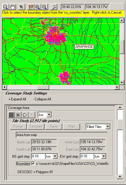

The yellow status bar across the top of the map will prompt you to select the desired object on the active layer. The tip set for the field on that layer will display the name of the object using the field you selected:
Click the object you want to use and the limits of the object will be displayed for the coverage area:
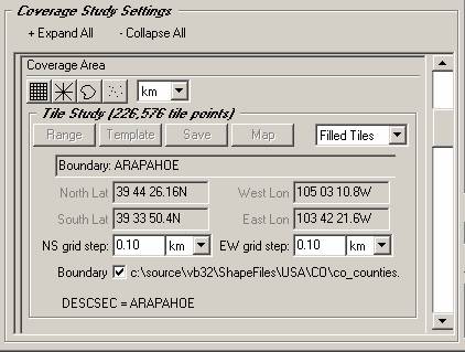
Note that the latitude and longitude limits are grayed-out and cannot be edited because the area is defined by the selected boundary. You can uncheck the Boundary box to use these limits but not the boundary polygon.
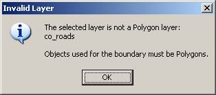
Boundary objects for tile studies must be polygon objects. Shapefiles also support point and line object (such as building locations or roads).
You can select a line or point layer to use the field tips on that layer:

However, if you click the Boundary checkbox to use an object on a point or line layer, a message will be displayed:
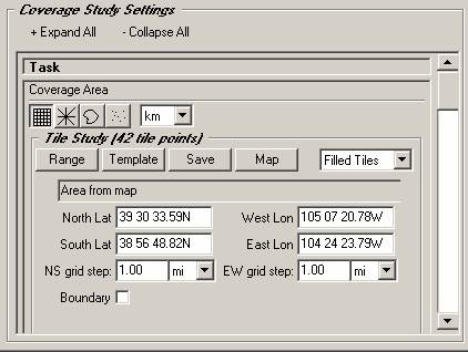
When the area limits have been set as desired (using any of the methods described above), you can also set the grid step value:
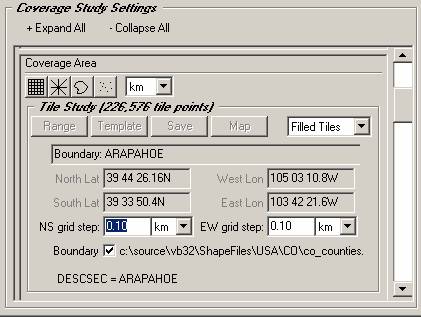
The grid step value determines the spacing of the computed points on the tile grid. Smaller step values result in more points and more detail but with longer execution times. Larger steps result in faster execution since fewer points are computed, but there is less detail and more visible "pixilation" of the tiles.
To create a Target study, click the button showing the individual points:
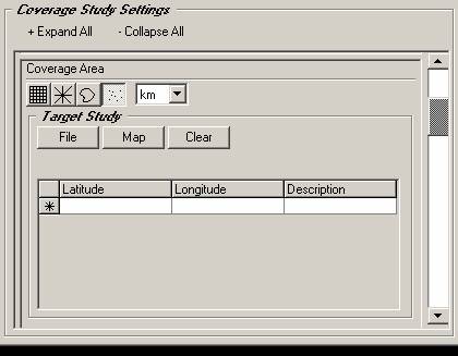

The form will display the Target settings.
(For importing Target Points from an Excel spreadsheet file, see the Target Point Study Import article.)
You can define Target points by scrolling (if necessary) to the end of the list to the row with the asterisk (“*”) in the selection button on the left of the row. When you start typing on that row, a new Target point record is created:
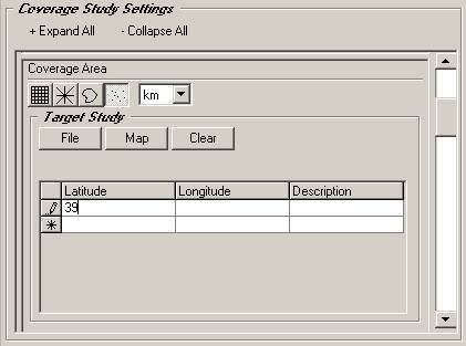

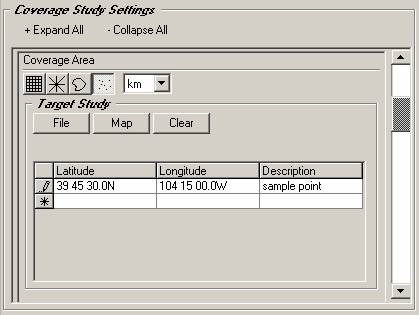
You can fill in the desired values in each column:

Note the pencil icon at the left end of the row indicating that the value is being edited. You can undo the edit as long as the pencil is displayed by clicking the Esc key on your keyboard and the original value will be displayed.
You can delete a row by selecting it by clicking on the selection button to the left of the row and clicking the Delete key on your keyboard.
Click another line to move off of the new line so the pencil icon disappears. This is necessary to be sure the new added point is saved.
You can add points from a shapefile by clicking the File button:
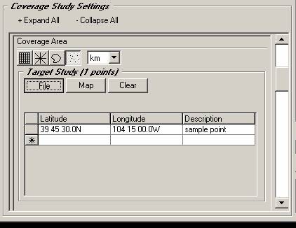

You will be prompted to select a shapefile:
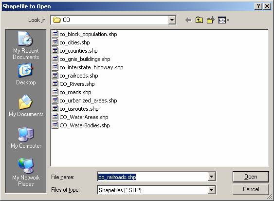
You can select any shapefile (polygon, line, or point). If a polygon or line file is selected, all of the points for each object in the file will be added, such as vertex points around a polygon object (like a county boundary) or points on a line (such as a road).
When you Open the file, you will be prompted to select a field in the shapefile:
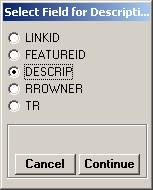
The field will be used for the Description column for the Target points.
When you click Continue the points will be added to the Target list:
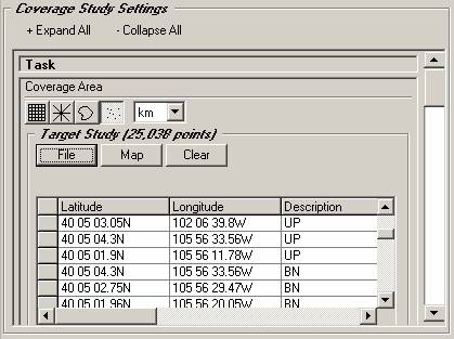

Note that for large shapefiles the process may take several seconds.
You can also add Target points from locations you click on the map. Click the Map button:
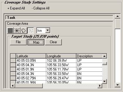

The yellow status bar on the map will prompt you to click on the map to get coordinates of points you want to add to the Target list:
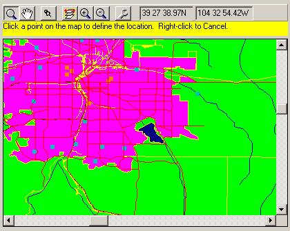

Each time you click the map, the coordinates of the point you click will be added to the Target list. You can add a description of the point:
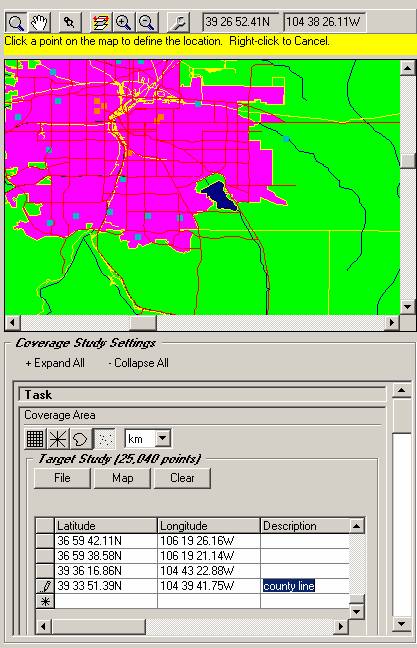

When you have finished adding points from the map you can right-click on the map.
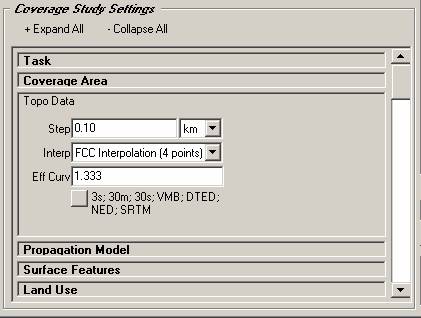
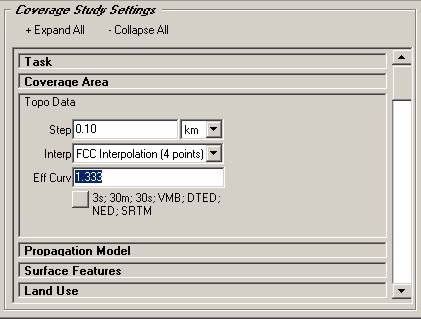
To change the topographic elevation data used on the path, click the Topo Data label to open the Topo Data section:
(Note that if the section you want displays below the bottom of the form, you can use the vertical scroll bar on the right of the list of sections to scroll up and down on the list.)
You can change the type of data used, or the increment (“step”) between the elevation points, the elevation interpolation method used, or the effective earth curvature used.
The Topo Data step is the increment between elevation points along a path from the fixed facility and the point where the field strength is to be computed.
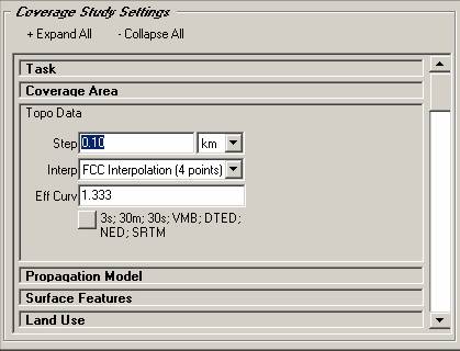

The step value should be selected to correlate with the type of topographic elevation data being used (discussed below). If the increment is set very large in comparison to the topo data resolution, much of the terrain detail could be missed. If the increment is set unnecessarily small, the processing time for the study may be significantly increased.
For example, if you have 1-second USGS NED (National Elevation Dataset) data for the coverage area it would make sense to set the topo data step to a value in the range of 30 to 50 meters. (The 1-second grid for the NED data in North America is about 30 to 50 meters.) If you set the step to 1-kilometer, the program will only retrieve elevation points along a path every 1-kilometer, ignoring much of the available detail in the NED data.
On the other hand, if you only have 30-second data for the area (with a resolution of about a half-mile for elevation values), setting the topo data step to 50-meters would result in a significant amount of processing time used to read elevations interpolated from the same data points. This will increase the time for the study without providing additional useful elevation data for the program.
In general, the goal is to avoid these extremes when setting the topographic elevation data step value.
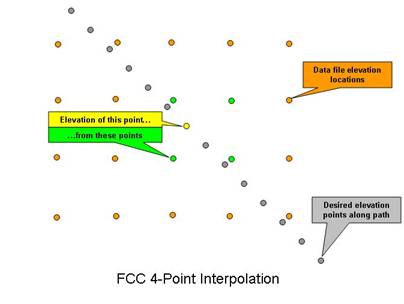
The interpolation method you select is used to determine elevation values at points along the path between the fixed facility site and the field strength locations.
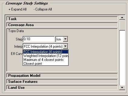
The topographic data files consist of elevations at locations on a uniform rectangular grid. Various interpolation methods are available for determining the elevation at points between these locations. For more information, see the article on Terrain Elevation Interpolation.
□ FCC-4 Point Method uses the four closest points. This is the method specified by the FCC in Public Notice 84-705, July 13, 1984:

□ Maximum Elevation Method uses the four closest points and selects the maximum elevation value. This method is typically used for checking microwave paths for worst-case clearance over a path.
□ Closest Point Method uses the elevation of the database point closest to the desire point. This method is slightly faster than the other methods but should only be used with higher resolution topographic data (30-meter/1-second or better.)
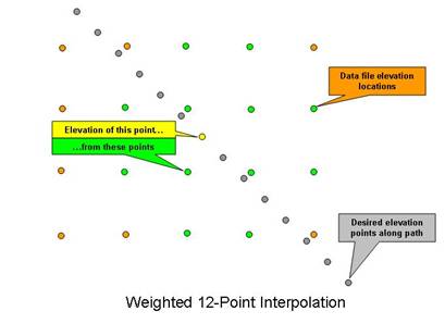
□ Weighted 12-Point Method uses the 12 closest points. This method considers additional factors, such as the slope of the terrain around the desired point. Since twelve points are required for each interpolated elevation (instead of the four points for the FCC interpolation) this method will be slower:

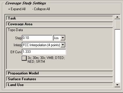
The effective curvature indicates the effect of atmospheric refraction on the radio wave propagation.
This value is typically set as 1.333 (“4/3 earth”), but you can set the effective earth curvature to any value greater than zero.
You can click the button to select the topographic data types to include:
When you click the button, the supported data types are displayed:
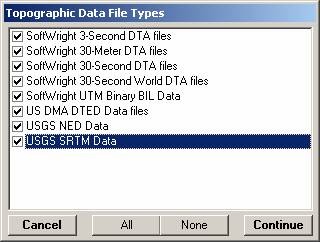
Naturally, the program will only use the data files that are installed on your TAP system. For more information about indexing data files, see the article on TopoScript Data Configuration.
Typically, you can select all the data types. The program will search the indexed data files and find the highest resolution data for each part of the area. For example, if you have 3-second data files for the entire area, and 1-second NED data for a portion of the area, the program will use the higher resolution 1-second data where possible, and the 3-second data everywhere else.
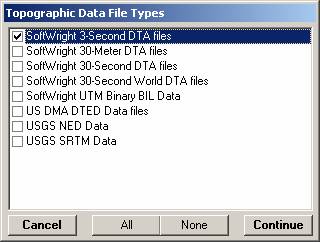
If you have a special requirement to use only certain types of data, you can uncheck the other types for the study:
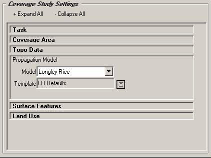
To select the propagation model or to change the model parameters you want to use, click the Propagation Model label to open the Propagation Model section:
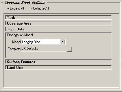
(Note that if the section you want displays below the bottom of the form, you can use the vertical scroll bar on the right of the list of sections to scroll up and down on the list.)
You can select the propagation model from the list that displays the models that are licensed to your TAP system:
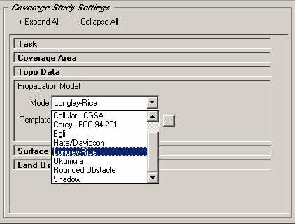
For more information on the characteristics of different propagation models, see the article on Propagation Models.
Each propagation model has different parameters and settings that you can use to control how the calculations are performed. These settings are contained in Templates you can view, edit, or create by clicking the Template button:
When you click the Template button, the Template database for the selected propagation model is displayed:
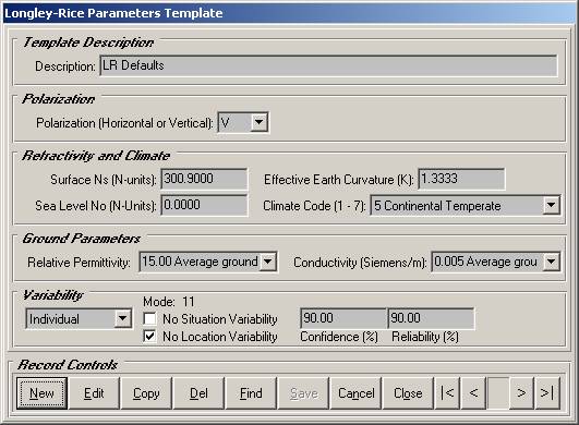
Note that the template layout and parameters will be different for each propagation model.
To change the Surface Feature files used on the path, click the Surface Features label to open the Surface Features section:
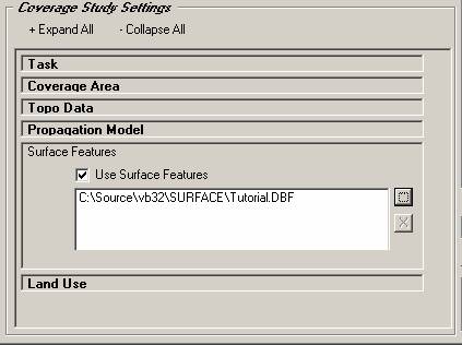
(Note that if the section you want displays below the bottom of the form, you can use the vertical scroll bar on the right of the list of sections to scroll up and down on the list.)
You can choose to ignore Surface Feature files by un-checking the “Use Surface Features” box.
You could also use the “X” button to remove selected Surface Feature files from the list. The “…” browse button is used to add Surface Feature files to the list.
Surface Features are described in more detail in the article on Surface Feature Files.
To change the Land Use features used on the path, click the Land Use label to open the Land Use section. (This section will only be available if the Land Use module is licensed to your TAP system):
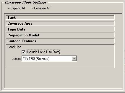

(Note that if the section you want displays below the bottom of the form, you can use the vertical scroll bar on the right of the list of sections to scroll up and down on the list.)
The Land Use data are files created from the USGS Land Use Land Cover files based on 1:250,000 scale maps. The files are based on a with a classification value assigned to each 200x200-meter area. The classifications indicate the general characteristics, such as Industrial or Forest.
The pull-down list indicates the loss template to be used in computing signal loss values at locations based on the transmit frequency and Land Use code at each location. The templates correlate various frequency ranges and Land Use classifications, and a loss value (in dB) for each combination. (Some of the templates have gaps for some frequency or Land Use classifications, but the software includes an editor so you can modify or create your own values or even your own templates. For more information, see the article on Land Use Data.
If the “Include Land Use Data” box is checked the program will find the USGS Land Use classification for each location where the field strength is computed. If the selected template includes an entry for the frequency (from the Fixed Facility) and the Land Use category (from the Land Use file), that loss value will be applied to the computed field strength at that location.
For example, suppose the computed field strength at a location is 42dBu, and the Land Use classification at that location is Agricultural (Land Use code 21). If the operating frequency is 455MHz and the “TIA TR8 (Revised)” template was selected, the loss value for that frequency and Land Use is 4dB, so the computed field strength saved by TAP would be 38dBu (42dBu minus 4dB).
You can also create your own files as described in Creating Land Use Files.
Several Loss Templates are provided with the software. These are described in the Land Use Data article. You should evaluate the templates to determine which is most applicable to your work.
To view or edit the Task information, click the Task label to open the Task section:
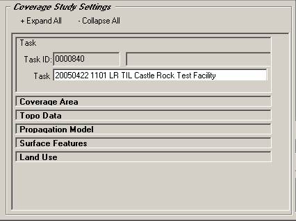

Each coverage study in TAP is assigned a “Task” ID, a seven-digit numerical “key” that TAP uses to identify files and other components needed for that study. The Task ID cannot be changed by the user.
The Task also has a Task Description that you should enter to help you locate or identify the Task later. If the Task Description is blank and you double-click the Description section, the program will attempt to create a description with the date and time (to ensure a unique Task Description), and other information from the form, such as the propagation model and type of study, as well as a description of the fixed facility site being used. You should only do this after you have set the parameters. If you change the parameters the Task Description is not automatically changed. You can, however, go back and remove the description, then double-click to create a new description, or you can edit the description manually.
If you want to automatically draw the coverage map after the study has completed, mark the “AutoDraw”checkbox:
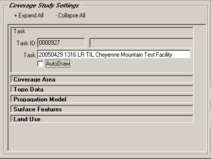

When the box is checked, the study will be plotted in HDMapper™ when completed. If you are running multiple studies, each will be plotted as soon as it is finished. If you are running a large number of studies you may not want to plot them all automatically. The area of the screen and the memory and other resources of your machine may not be adequate to usefully display more than a few maps.
Create a new task by clicking the blank document button on the toolbar near the top of the HDCoverage form:
The program will assign a new Task ID. After you have set the study parameters, Fixed Facility, Mobile Facility, etc., you can save the Task.
When you have set the parameters for the study you want to run you can save the study by clicking the Save button on the toolbar near the top of the form:

The Task and its settings will be saved.
If you want to open a previously created Task, you can use the Open button on the toolbar near the top of the form:

When you click the button, you will be prompted to select the Task you want to open:
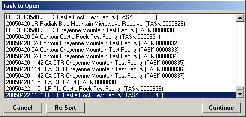
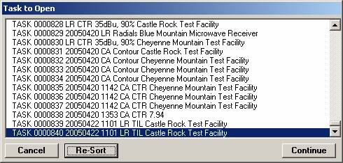
The Re-Sort button can be used to toggle between a sort by Task Description and a sort by Task ID:
Select the Task you want by clicking it to highlight that line and click the Continue button. The selected Task will be opened in the HDCoverage form.
Some Tasks are “Locked”. When a Task is run, the results of that coverage study are written to a file for use by TAP to plot the study and other functions. If the parameters of the Task were edited it could lead to confusing ambiguity. For example, suppose a coverage study was run with an ERP of 100Watts and the results were plotted. Then later the study parameters were changed to an ERP of 500Watts. The result would be an inconsistency between the parameters of the Task and the computed results.
For this reason, once a study has been run it is Locked. When you open a Locked Task, the status is displayed:
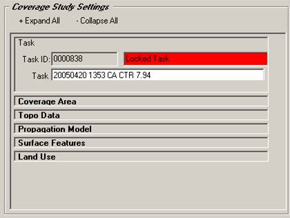

You will be prompted with the option to use the parameters from the Locked Task to create a New task
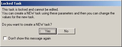
The new Task will have all the same parameters but a new Task ID. This Task can be edited and then run to produce a new coverage study with the new parameters.
This function enables you to recreate a Task with only slight changes (such as changing the ERP in the example above).
When you are ready to execute a Task to compute the coverage, click the Run button on the toolbar near the top of the form.

A list will be displayed showing all of the Tasks available to be run. (Locked Tasks that have already been run are not listed.)
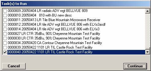
All the Tasks which you have edited during this session will be marked with a check. You can check or uncheck any of the boxes to select the list of Tasks you want to run.
When you have selected the Tasks you want to run, click the Continue button to start running that list of Tasks.
|
|
|
Copyright 2005 by SoftWright LLC