Yes, TAP can be used to design, study, and analyze P25 systems. Note that this example is for illustrative purposes only. Use the system configuration information and RF settings appropriate for your system and your RF environment.
The objective of Project 25 (P25) is an evolving, open digital radio standard for public safety that enables interoperability across government agencies without constraining vendor selection within respective government jurisdictions [1]. P25 represents a partnership between government and industry. Interoperability between different vendor hardware is ensured through the development of P25 communication standards and protocols by the Telecommunications Industry Association (TIA) in response to user-driven requirements. Manufacturers develop hardware that conform to these standards and submit them to compliance testing, while the responsibility for the specification and operation of individual P25-compliant systems resides with the user community [2]. SoftWright actively participates in the P25 process.
The development of P25 standards has facilitated the transition of public safety communication networks from analog to digital trunked systems, which provide improved bandwidth efficiency for voice channels and enable an expanded array of data services to meet a diverse set of user requirements. Adaptive modulation can support higher data rates in bandwidth- and interference-limited channels. Thus, coverage modeling of P25 systems must consider multiple channel types, hardware configurations, and tiers of service. For example, it may be necessary to determine the area coverage within a given jurisdiction for both voice and multi-rate data channels, both portable and mobile hardware, and both TalkOut and TalkBack (i.e., Forward/Reverse or Downlink/Uplink). TAPTM allows users to organize results to assess multiple combinations from a single set of area coverage studies.
The following is an example area coverage assessment for a P25 system. While parameters are based on values extracted from the FCC’s Universal Licensing System (ULS) database and hardware specifications, they should only be considered as example parameters and not an exact replication of a practical system implementation. This procedure is not intended to supplant a user’s required evaluation procedure, but should provide some guidance on undertaking the process in TAPTM.
Example P25 Coverage Requirement
Determine the area coverage for a P25 system operating in the 800 MHz public safety band in Albemarle County, Virginia, USA with the following parameters.
Base Stations
| Sites | Latitude | Longitude | Antenna Height | ERP |
|---|---|---|---|---|
| Carters Mountain | 37.98233º | -78.48236º | 76.2 m | 100 W |
| Fan Mountain | 37.87675º | -78.69086º | 36.7 m | 75 W |
| Bucks Elbow Mountain | 38.10458º | -78.74475º | 36.7 m | 100 W |
| Peters Mountain | 38.12286º | -78.29017º | 32.0 m | 100 W |
The same base station antenna heights are used for TX and RX. The antenna is omni-directional, with a gain of 12 dBi. The TX frequency is set to 855 MHz. The ERPs are set according to the values listed in the above table. For the RX parameters, 5 dB of implementation loss is included for all sites, and sensitivities are set to -123 dBm, which corresponds to the base analog and digital sensitivities (12dB SINAD and C4FM at 5% BER, respectively) for the Motorola GTR 8000 Expandable Site Subsystem. Post-processing of results could also incorporate the sensitivities for H-CPM at 5% BER and QPSK, 16-QAM, and 64-QAM at 1%BER, in addition to this base sensitivity.
Mobile Hardware
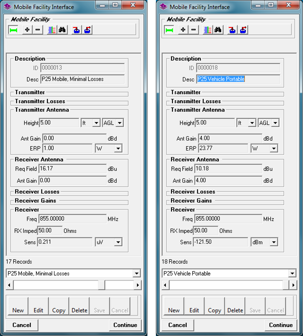
For the mobile unit, antenna height is set to 5 feet, with an antenna gain of 0 dBd. TX power is 1 W. No losses are assumed for TX. For the receiver, 3 dB of body losses are included. For a more conservative (e.g., indoor) assessment, additional body and building losses could be included. For the receiver sensitivity, we use values from the Motorola APXTM 8000, as shown here. The required field at the input to the antenna is also shown (as calculated automatically within the TAP mobile facility editor). (Note that the APXTM 8000 may alternatively be termed a portable or handheld, but is referred to as a mobile in the context of this example.)
| Requirement | Sensitivity | Required Field |
|---|---|---|
| Analog, 12dB SINAD | 0.236 μV | 17.15 dBu |
| Digital, 1% BER | 0.211 μV | 16.17 dBu |
| Digital, 5% BER | 0.178 μV | 14.70 dBu |
Portable Hardware
A mobile facility for a vehicle portable is also included. Antenna height is set to 5 feet, with an antenna gain of 4 dBd. TX power is 15 W. 2 dB of losses are assumed for TX and RX. For the receiver sensitivity, we use values from the Motorola APXTM 7500 Mobile, as shown here. The required field at the input to the antenna is also shown (as calculated automatically within the TAP fixed facility editor). (Note that the APXTM 7500 may alternatively be termed a mobile, but is referred to as a portable in the context of this example.)
| Requirement | Sensitivity | Required Field |
|---|---|---|
| Analog, 12dB SINAD | -121 dBm | 10.68 dBu |
| Digital, 5% BER | -121.5 dBm | 10.18 dBu |
Procedures
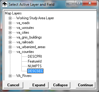
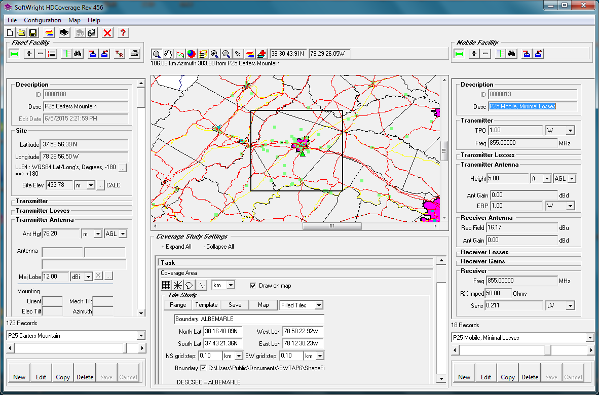
This analysis requires running four area coverage studies using HDCoverage. To start, generate a new study and give it a description that includes the name of the first site, “P25 Carters Mountain Albemarle Tile.” Create a new fixed facility named “P25 Carter Mountain.” Enter the fixed facility data, as described above, and save. After the save, TAP automatically loads the shape files for the state of Virginia. Click on the pin button to show the facility site and zoom to view Albemarle County. Right-click on the graphic to open the “Select Active Layer and Field” window. Select DESCSEC under va_counties.
Bounded tile studies will be used. Under the Coverage Area section, click on the tile button (the far left of the four). Click the box next to Boundary, and left-click inside Albemarle County in the graphic. You will see “DESCSEC = Albemarle” under Boundary, indicating that the boundary used for the bounded tile study will be the outline of Albemarle County. Set the NS and EW grid steps to 0.1 km, same as the topo step. The number of tile points will be updated – 341,264 unique study points to cover the county.
To keep this example simple, we do not include land use or surface features. For the propagation model, we use Longley-Rice, with default parameters. Users should set the propagation model and parameters to match their requirements and local RF environment.
Create, populate, and save new mobile facilities named “P25 Mobile, Minimal Losses” and “P25 Vehicle Portable” according to the parameters discussed above. (We also built a third mobile facility named “P25 Mobile, Severe Losses” that includes building losses and additional body losses, but it is not included in this example.) We will use “P25 Mobile, Minimal Losses” for the studies, so leave that mobile facility active. When the all of the study parameters are set, click on the Save button to save the study.
For each subsequent study, first click on the New button to create a new study. This will make an exact copy of the current study. Change the description to reflect the fixed facility being used (e.g., “P25 Fan Mountain Albemarle Tile”). Since the study is being run over the same area, with the same study parameters, no further changes are required under the “Coverage Study Settings” section. In the Fixed Facility Editor section, click on Copy to create a copy of the P25 Carters Mountain facility. Change the description to “P25 Fan Mountain,” enter the latitude/longitude and recalculate the site elevation, and set the TX and RX antenna heights and ERP. Save the facility. Then save the study. Repeat this process to set up studies for the “P25 Bucks Elbow Mountain” and “P25 Peters Mountain” sites.
After all four studies have been saved, click on the 6.3 button to run the studies. Be sure that all four studies are selected for the batch run and click Continue. The 6.3 progress window will open and show the progress of the studies. When the studies have completed, an HDMapper window will open with the coverage results of each of the four studies.
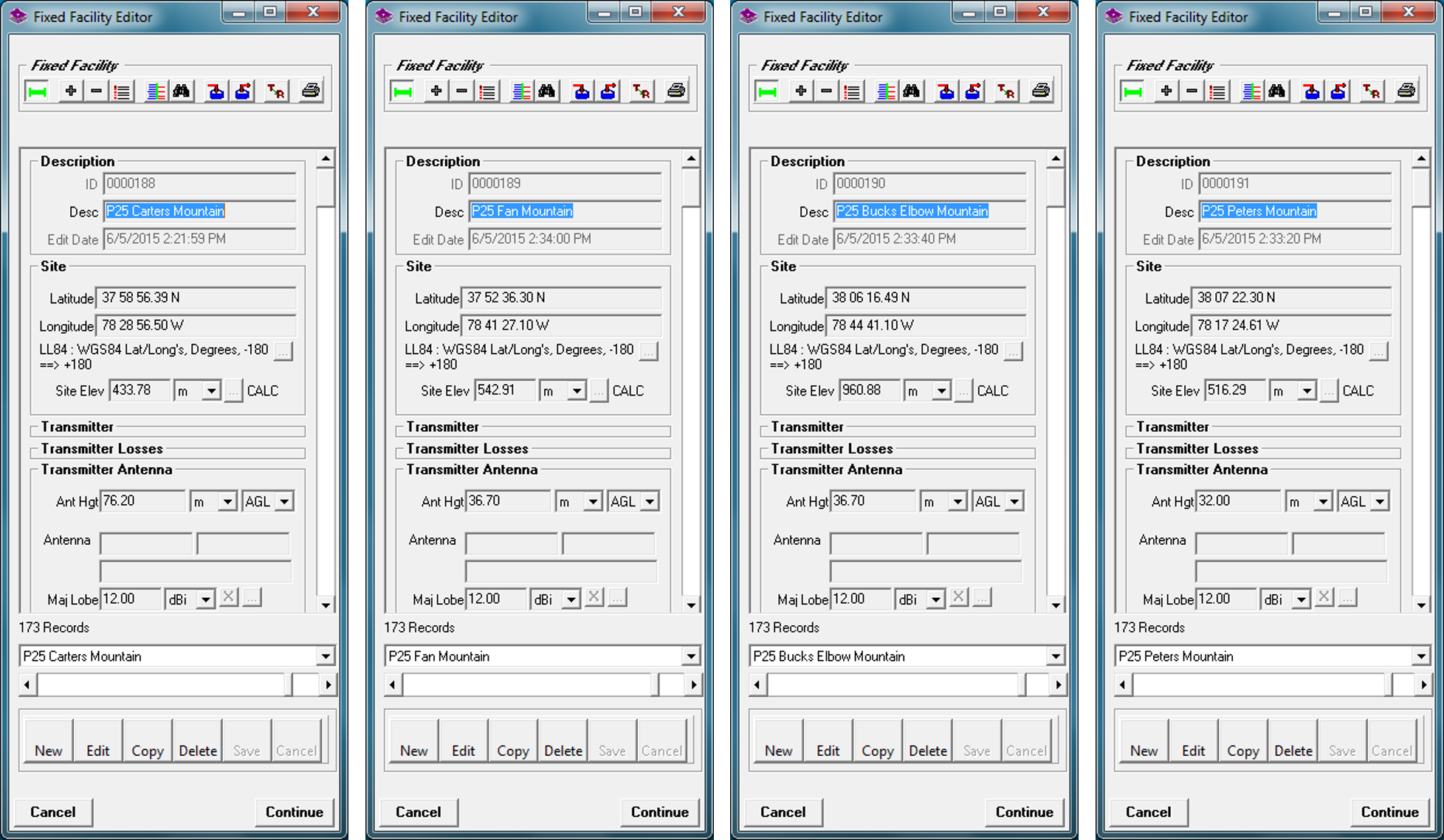
Fixed Facility Setup
After the studies have been set up, the fixed facilities should appear as shown here. Alternatively, one could set up all of the fixed facilities prior to setting up the four studies.
Mobile FACILITY SETUP
After the studies have been set up, the mobile facilities should appear as shown here.
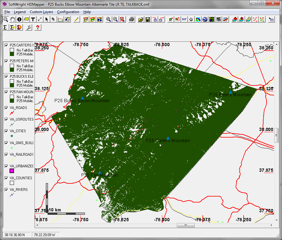
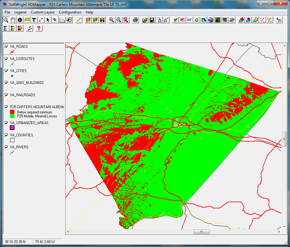
Coverage Study Results
When the coverage results for the individual studies initially load in HDMapper, the areas with received signal strength above threshold will be green. Areas below threshold will be red. The initial result for Carters Mountain is shown here.
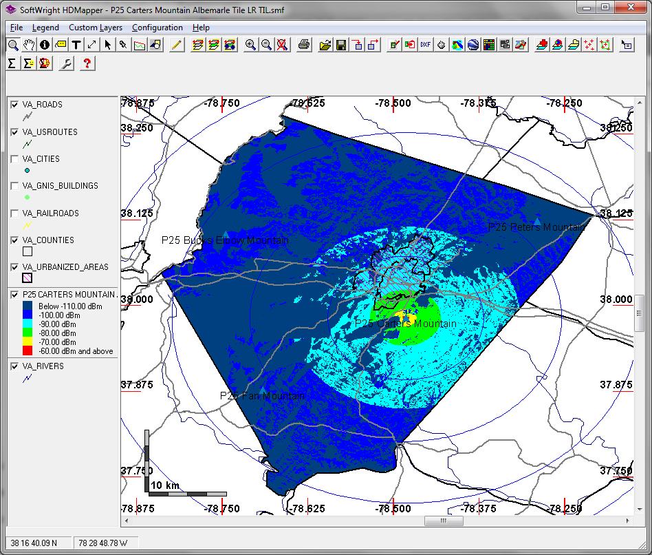
There are numerous options for adjusting the appearance of the coverage results. Shape file layers can be added and removed, and their order changed. The following figure shows the Carters Mountains results with several adjustments. The order and properties of the va_* shape files have been modified. Fixed facilities, Lat-Lon Tics, MapScale, and Distance Circles have been added. The coverage display was changed to dBm increments (by right-clicking on the coverage layer and selecting “Show dBm increment levels”).
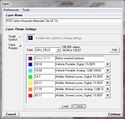
To view the coverage for the respective hardware performance levels, first disable “Show dBm increment levels.” Then double-click on the coverage layer to open the Layer Settings window. Initially, only two layers will be shown.
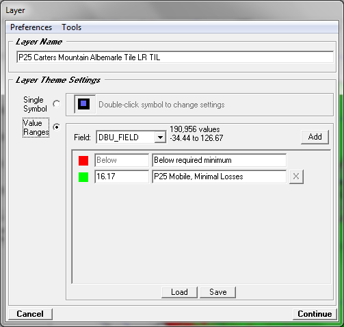
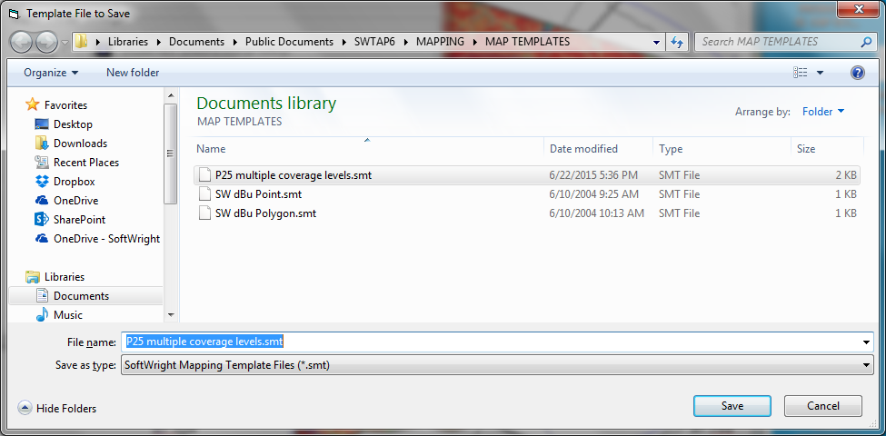
Use the Add button to add dBu thresholds and assign labels and colors, as desired. Our selections are shown in the following figure. If you will want to re-use these levels and layer settings for another study, click on the Save button to save the template, as shown here.
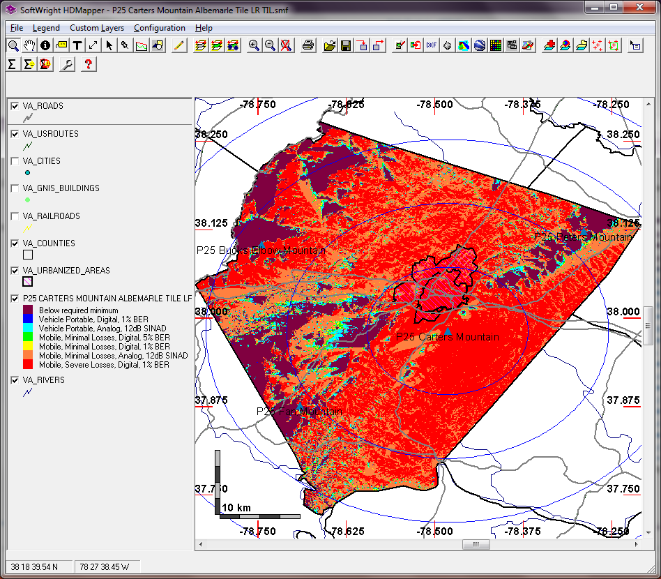
The multi-level coverage plot will appear as shown here. Note that the thresholds for the vehicle portable and the mobile are each tightly grouped, so that some of the areas are fairly small.
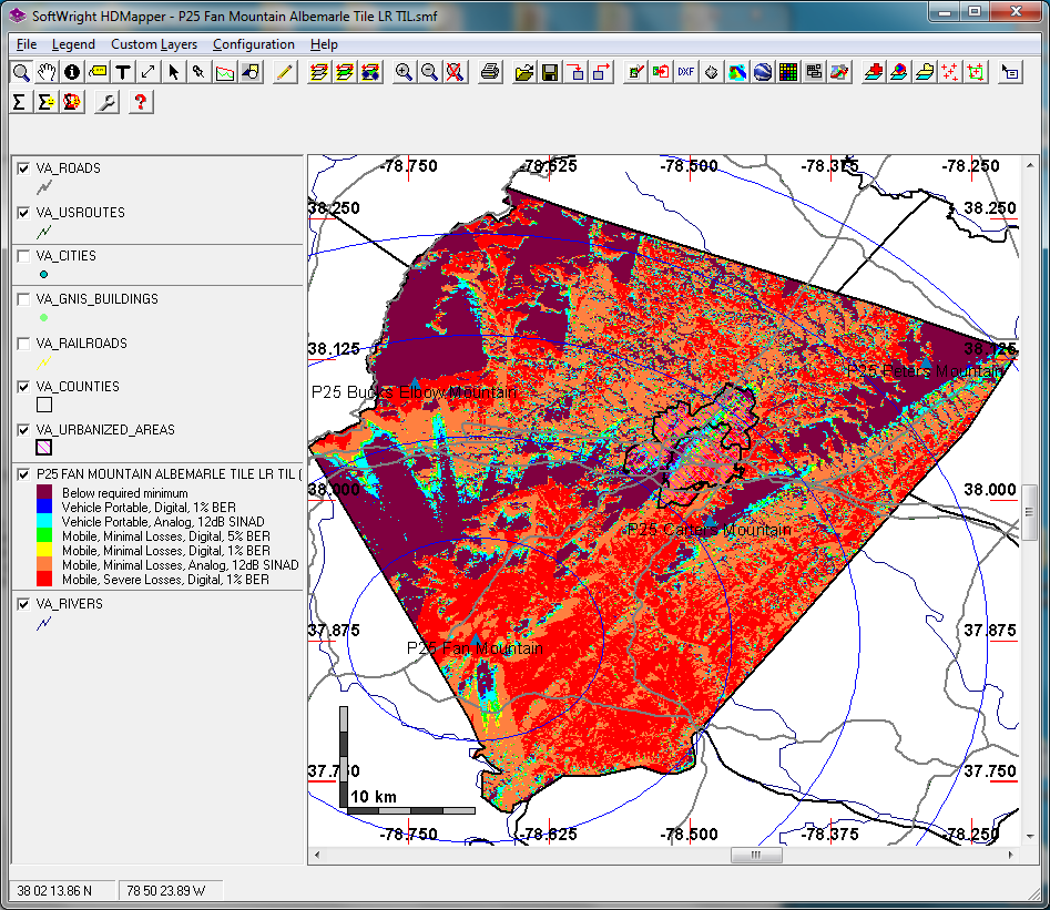
You can repeat the same process with the other sites, as desired. When opening the coverage layer, you can simply press the Load button and load the saved coverage levels template. Here is the same plot for Fan Mountain.
At any point, the Google Earth button can be used to create a KML file with the area coverage image, which can be viewed in Google Earth, or any other rendering program.
Composite Study
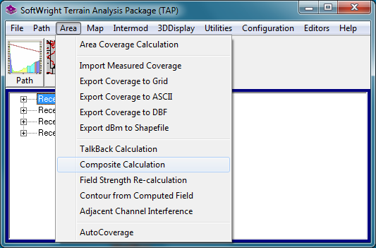
To assess the combined coverage of all four sites over the county, you can use the Aggregate Coverage module. On the main screen, select Area | Composite Calculation.
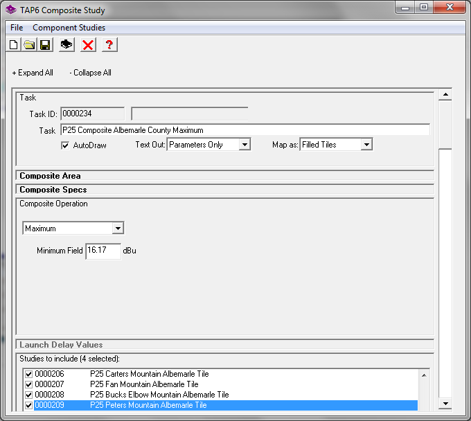
Click on the New button to create a new study. Name the study “P25 Composite Albemarle County Maximum.” Under the “Studies to include” section, select the four individual studies. Under the “Composite Area” section, click on the “Get Limits from studies” button and set the NS and EW grid steps to 0.1km. Under the “Composite Operation” section, select Maximum. Double Click on the Minimum Field value. This opens the Mobile Facility Editor. Select the “P25 Mobile, Minimal Losses” entry and Continue. The dBu value for this facility is now entered as the minimum field. Click Save to save the study setup and Run.
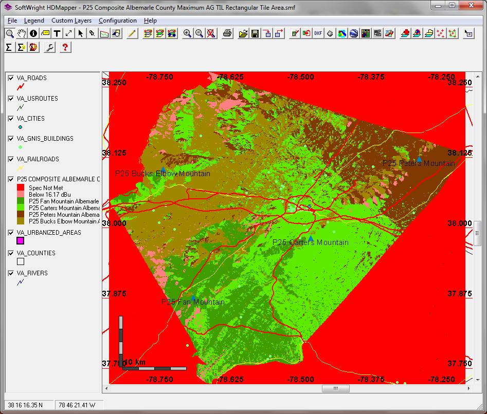
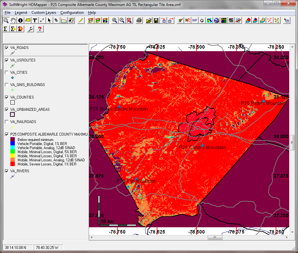
When the study completes, HDMapper will open, showing the results. The initial coverage map indicates the site providing the maximum signal strength (above threshold) at each study point. The red indicates areas not included in the component studies. The pink indicates areas where no sites supply an above-threshold signal. The areas covered by the different sites are color-coded.
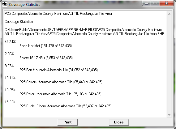
Right-click on the coverage layer and select Coverage Statistics. This determines the coverage statistics over the area. Note that the total number of points includes points outside the county. The other ratios need to account for the fact that only 342,435-151,479=190,956 of the points reside within the county. So:
Below 16.17 dBu: 6,853/190,956 = 3.59% (Thus, inversely, 96.41% of the county is covered.)
Fan Mountain: 31,052/190,956 = 16.26%
Carters Mountain: 65,448/190,956 = 34.27%
Peters Mountain: 35,106/190,956 = 18.38%
Bucks Elbow Mountain: 52,497/190,956 = 27.49%
To view the multi-level coverage over the area, right-click on the coverage layer and select “Show Composite as Multi-level Plot.” This loads the Layer Settings window with no thresholds listed. Click on Load and select the template that was saved earlier. Click Continue. Adjust the other shape file layers, as desired.
Checking the coverage statistics for the multi-level plot yields the percentage of the county covered at the different performance levels:
Vehicle Portable, Digital, 1% BER: 10.18dBu: 187,080/190,956 = 97.97%
Vehicle Portable, Analog, 12dB SINAD: 10.68dBu: 186,887/190,956 = 97.87%
Mobile, Minimal Losses, Digital, 5% BER: 14.70dBu: 185,036/190,956 = 97.30%
Mobile, Minimal Losses, Digital, 1% BER: 16.17dBu: 184,103/190,956 = 96.41%
Mobile, Minimal Losses, Analog, 12dB SINAD: 17.15dBu: 183,323/190,956 = 96.00%
Mobile, Severe Losses, Digital, 1% BER: 43.17dBu: 152,729/190,956 = 79.98%
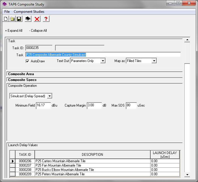
The results above were all for the Maximum composite operation. To do a simulcast study, simply open the previously-run composite study and click on the New button. This creates an identical copy of the previous study. Change the task description to “P25 Composite Albemarle County Simulcast.” Under Composite Operation, change the operation to Simulcast and set the capture margin and the maximum simulcast delay spread (80 μs, in this example). Note that the “Launch Delay Values” section becomes active and the delay values for the individual base stations can be set. Save and Run. Other operations include Best Server (i.e., setting only a capture margin) and D/U Ratio, which allows the user to conduct interference studies, if desired.
TalkBack
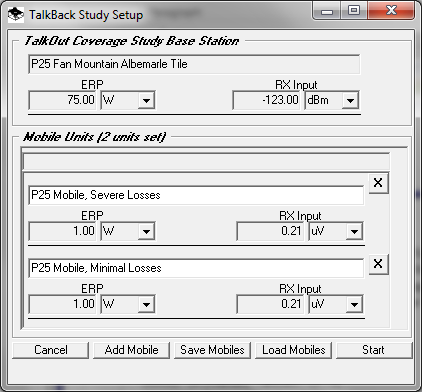
There are multiple options to assess the TalkBack coverage over the area. The simplest approach is to select Area | TalkBack calculation from the main menu. Select the study on which to perform the TalkBack calculation. This opens the TalkBack Study Setup window. Multiple mobile units can be selected for the TalkBack study. In the case, we just select “P25 Mobile, Minimal Losses” and Start the study. We repeat this for the other sites as well.
Once all of the TalkBack studies have completed, they can be overlaid on a single plot, and manipulated from there to achieve the desired appearance. There are a number of other options for creating and viewing TalkBack coverage in TAP, depending on the system parameters.