TAP includes two approaches to these multi-site calculations:

• Aggregate Coverage is more exact, since all calculations at target points in the area from each of the base stations are computed at exactly the same target points. However, this imposes the limitation that the original study from each site is performed for exactly the same area. This may not be realistic for a study over a large geographical area involving numerous, widely-separated base stations. Only Tile studies can be used.
• Composite Coverage permits the use of any tile or radial studies computed with TAP, over any region. The computed values from each study are compared with any values from other studies within a user-defined "search radius", and uses the geographically closest value from each site for the calculation of the resulting value at that location.

For example, suppose you have computed two coverage studies, a tile study from the sample Castle Rock site (used in the TAP demo and tutorials), and a radial study from the Cheyenne Mountain site (also used in the demo).

Plotting a field level (for example, 20dBu) from multiple sites with a different color for each site results in a map as shown below:

If you want to examine the coverage in the overlapping area (such as the highlighted Douglas County), you can use the TAP Composite Coverage function to combine the two studies. (If you wanted to use the TAP Aggregate Coverage function you would need to compute new studies from each site over the area of interest to meet the more strict requirements of Aggregate Studies as described above.)

The Composite Coverage function is executed from the Coverage menu in TAP:

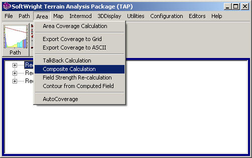
If you are using TAP5 or earlier, the menu will be as shown below:

When you click the menu, the TAP Composite Study form is displayed:

To create a new Composite Study, click the New button. A new Task ID will be assigned by the program in the box in the upper right corner of the form.

Enter the information on the form for the study you want to perform:

Study

Enter a description of the study. This description will be used later when you want to select the study to plot. You can leave the study description blank, and after you have set all the study parameters as described below, double-click the description text box to assign a description based on the date (year,month,day) and the type of study.

Composite Specifications

Specify the area for the study. You can define the study area as a rectangular area or a polygon that is defined by a boundary file.

For a rectangular area, you can enter the north, south, east, and west boundaries manually, or you can use the TAP Area Template database. The Area Template database enables you to define an area that you may want to use in several studies and save those parameters.

For example, click the Template button:, and the Area Template database will be opened:

Use the Find button to locate the template you want, or the New button to define a new template:

When you Close the Area Template form, the area limits are written to the Composite Study form:

For this example, we will use the other option, an area defined by a boundary file.

Click the Use Boundary box:

When you click this box, the Select Boundary File Object dialog box is displayed:

This form enables you to select an boundary (.BNA) file (such as Co_hires.bna in this example). When you select a file, the objects in the file are displayed. Then you can select the object (such as "Douglas" in this file). You can use the TAP Boundary File Editor to create your own areas in the .BNA format.

Click the Continue button on the Select Boundary File Object form. The boundary limits from the selected object will be displayed on the Composite Study form.

(The coordinate text boxes are disabled, since the values are determined by the selected object.)

Set the Grid Step (such as 0.5 mi in this example). This determines the spacing of points within the area (rectangular or boundary file).

When the study is executed, each computed field strength point for each study selected (as described below) will be used as a target point for computing the Composite value (based on the operation specified). The value for that point will be considered along with the closest point from each other study that is within the Grid Step distance. This means if you specify a grid step of 0.5 mile as in this example, points as far apart as one mile (i.e., points from two other studies, each a half mile on opposite sides of the target point) will be used together.

Select the option of Field Strength Studies or Shadow Studies. The Composite Study can be used with Shadow studies to determine the best line of sight to each location from multiple transmitter sites.

If you want to combine the results of other Aggregate or Composite studies in this Composite study, check the box on the form.

Composite Operation

Select the operation to use with the points from the different coverage studies. The Maximum option simply selects the highest of the field strength (or shadow ratio) levels.

For this example, select the Best Server option:

The Best Server option selects the highest field level as long as it exceeds the second highest level by at least the value specified as the Capture Margin. If the Capture Margin specification is not met, a value of -32000 is written for the value at that location.

When Best Server is the selected option, you can enter the Capture Margin value:

Tasks to Include

The list near the bottom of the form displays Tile and Radial studies computed in TAP. The list will be refreshed if you change the "Field or Shadow" option, or the "Include Aggregate…" option.

Click the checkbox at the left of the lines for each study you want to include.

You can right-click on a highlighted line to display a summary of that Task.

(Note that the summary is displayed for the highlighted line even if you click elsewhere on the list.) Click the checkbox at the left end of a line to include the results of a study in this Composite Coverage.

If you left the Task Description blank, you can double-click the description text box to insert the automated information:

You can edit the description that is created:

When you have specified the parameters for the Composite Study, click the Start button at the lower right of the form (or click the Cancel button to abandon the operation):

A progress form will be displayed as the study runs:

Note that the progress of the study will not be linear. In areas of overlap between two or more studies, the progress will be slower. In areas where only one study is being considered (i.e., outside the range of any other study) the progress will be much faster. Therefore any "Time remaining" information displayed (after the 10% progress is reached) will usually not be accurate for Composite Studies.

When the study is completed, you can use the File-New Map menu to draw the results:

The Map Plot Setup form will be displayed. Use the Add button in the Coverages section to add the Composite Coverage study to the plot:

A form will be displayed listing the available Tasks that can be plotted on the map. Select the Composite Coverage study. (Note the Results section of the form shows the Composite Coverage as an "Aggregate Study". This is because the results are saved and plotted in the same way as Aggregate studies.)

The Tile and Radial studies that were included in the Composite study will be shown on the Map Plot Setup form.

You can select each of the individual studies and double-click the line to set the color for that study.

For Aggregate and Composite studies, you will normally assign a different color to each study so the map will show the points served by each different study by using the color for that study.

To set the field strength (or shadow ratio) level for the map, click the Field Levels (or Shadow Levels) button on the Map Plot Setup form.

The Levels form will be displayed. For Aggregate or Composite studies, be sure the "Plot a single level…" box is checked. Then you can select a single level from the list of values. That is the level that will be used to plot the resulting value at each location, using the color corresponding to the site providing the service to that location. Use the option buttons at the left of the list to select the level you want to plot.

The coverage will be plotted in the TAP Map Window.

In this example, you can see that coverage from the Castle Rock site (the Tile study to the north) is plotted in red, and the coverage from Cheyenne Mountain (the Radial study to the south) is plotted in green. Since this is a Best Server study, there are several areas showing no coverage, usually indicating that the Capture Margin requirements were not met for those points.

The same study could be set up and run to display the Maximum coverage:

In this case, the resulting Composite Coverage is shown with all locations plotted either in red (the maximum signal is from the Castle Rock site) or green (maximum from the Cheyenne Mountain site).