Composite Studies in TAP6
Q: How can I show coverages from multiple sites over an area, including regions where the coverages overlap?
A: In TAP 6 systems licensed for the Aggregate Coverage module with TAP version 6.0.2105 or higher and with a Maintenance Subscription date of August 31, 2006, or later, you can use an improved version of the Composite Study function.
Other topics of interest for Composite studies:
Aggregate Coverage Demonstration
How can I make my Composite studies run faster?
How do I compute an interference study in TAP?
This version of the Composite Coverage function includes several features not present in the earlier version, such as the ability to save and load Composite studies, and the ability to run several Composite studies in a "batch" mode.
For example, suppose you have computed two coverage studies, a tile study from the sample Castle Rock site (used in the TAP demo and tutorials), and a radial study from the Cheyenne Mountain site (also used in the demo).
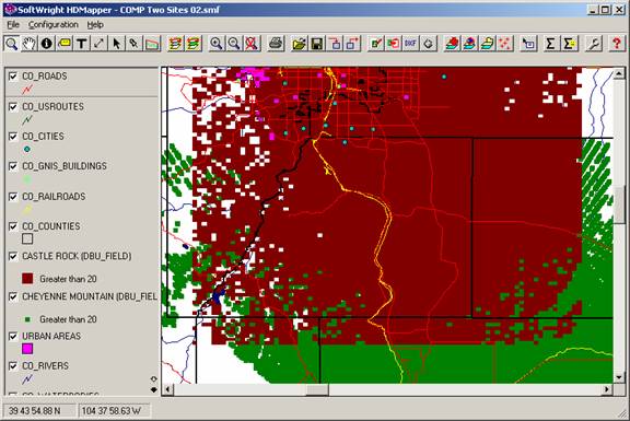
Plotting a field level (for example, 20dBu) from multiple sites with a different color for each site results in a map as shown below:
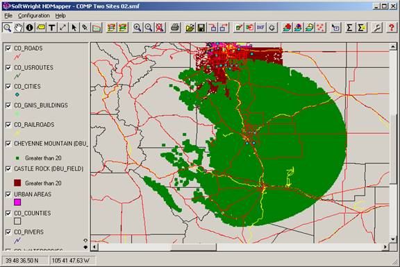
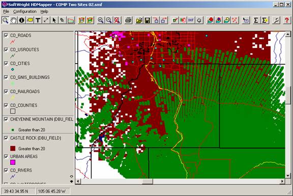
You can change the layer order on the HDMapper form to see the two overlapping coverage areas:
In order to see the results of combining the two computed coverages together mathematically, you can use the TAP Composite Coverage calculation.
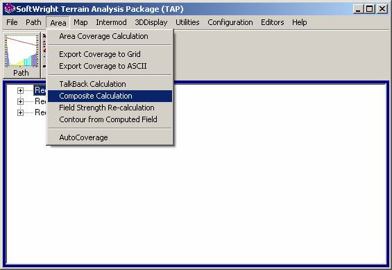
From the TAP6 menu, select the Area menu, then click Composite Calculation:
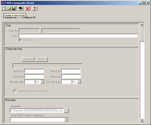
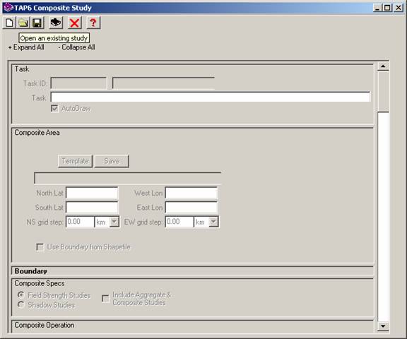
The TAP6 Composite Study form will be displayed:

To create a new study, click the New button at the left end of the toolbar near the top of the form:
A new Task ID is assigned by the program:
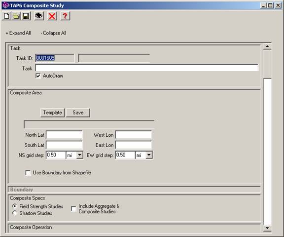
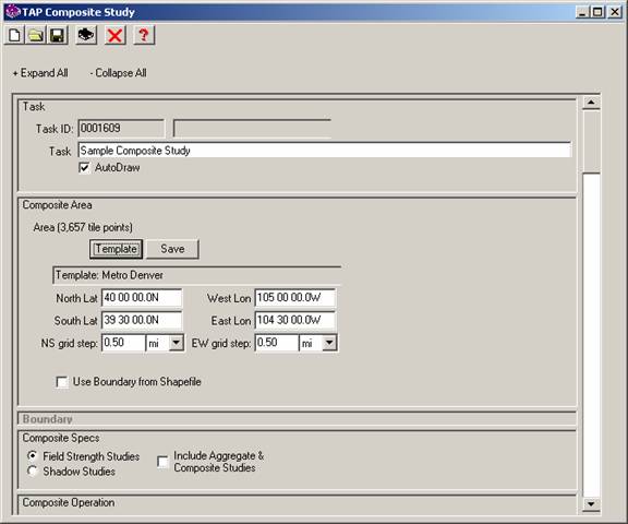
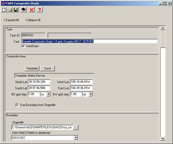
Task
Enter a description of the study.
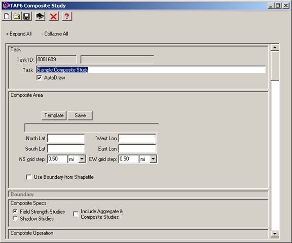
This description will be used later when you want to select the study to plot. You can leave the study description blank, and after you have set all the study parameters as described below, double-click the description text box to assign a description based on the date (year,month,day) and the type of study.
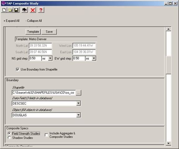
Composite Area
Specify the area for the study. You can define the study area as a rectangular area or a polygon that is defined by a boundary contained in a shapefile.
There are several options for defining the area where the composite calculations are to be performed:
□ For a rectangular area, you can enter the north, south, east, and west boundaries manually
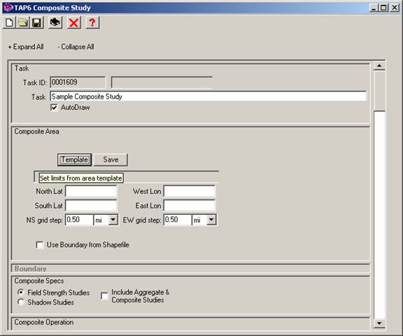
□ You can use the TAP Area Template database. The Area Template database enables you to define an area that you may want to use in several studies and save those parameters.
□ You can use a boundary from a shapefile to compute the composite values in an irregular area, such as a county.
For example, click the Template button:
The Area Template database will be opened:
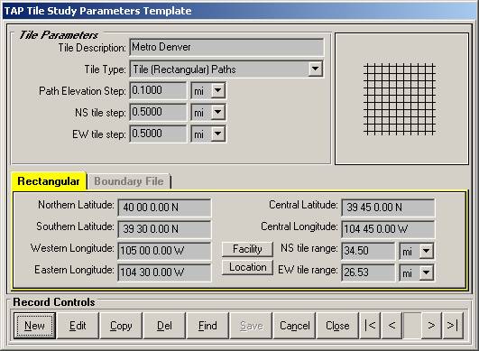
Suppose you want to compute the composite of the two coverages in the area defined by this sample template, “Metro Denver.” Click the Close button to bring the rectangular limits back to the Composite Coverage form:
You could use these setting to compute the coverage where the two studies overlap the specified rectangular area.
For this example, we will use the other option, an area defined by a boundary file. Click the Use Boundary box:
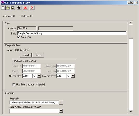
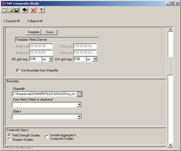
When the “Use Boundary from Shapefile” box is checked, the Boundary section of the form is enabled. This section enables you to select a file, a data field in the file, and an object to use.
For example, use the lookup button (“…”) to the right of the Shapefile box to lookup a shapefile:
Use the Open dialog box to find the Shapefiles folder where TAP is installed and select the file in the CO (Colorado) folder for the Colorado Counties (co_counties.shp):
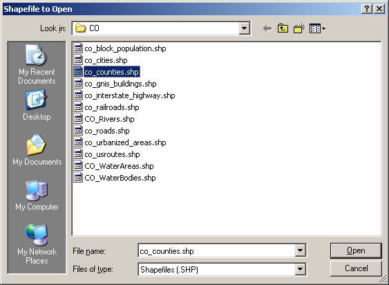
The shapefile you select must contain polygon objects. The other two possible shapefile types (line objects or point objects) cannot be used with this function.
When the shapefile has been selected, use the pulldown list to select the data field to use.
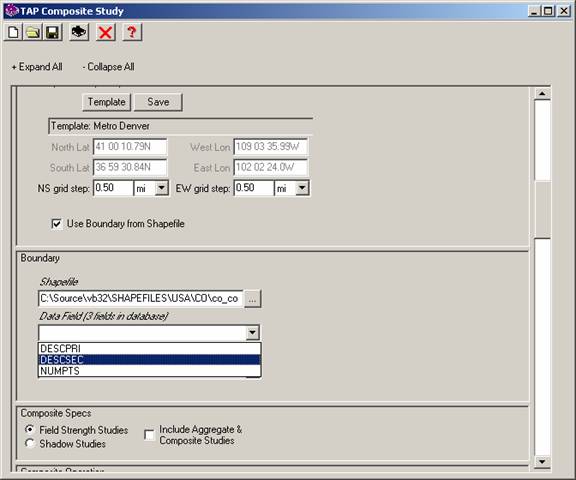
For this example, select the DescSec (“secondary description”) field.
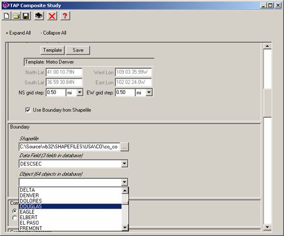
The data field selected will be used to identify which object (see below) from the file you want to use.
Shapefiles can have a wide variety of data fields (one of the powerful attributes that make shapefiles so flexible). The field you select with other shapefiles will depend on the file. For shapefiles from other sources, you should contact the source of the file to determine the contents of each of the data fields.
When the desired data field has been selected, a list of the value in that data field will be displayed for all the objects in the file. For this example, select the Douglas county object:
After you have selected the object, note that the North, South, West and East boxes have been disabled. Since you are defining the area from a shapefile (the Use Boundary box is checked) you cannot change the coordinates. If you want different coordinates you must uncheck the Use Boundary box.
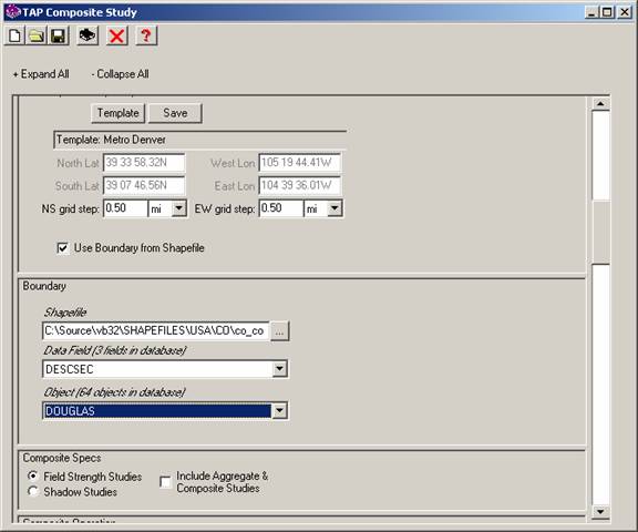
Note also that the coordinates in the boxes have been changed to represent the bounding coordinates for the selected object (in this case, Douglas County).
Select the grid step in the area. This defines the rectangular grid where the program will compute the composite of the studies from the different sites. For this example, use a step value of 0.5 miles.
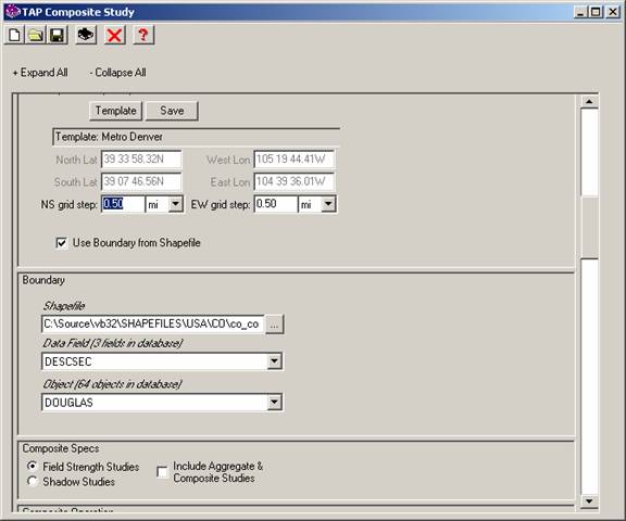
When the study is executed, each computed field strength point for each study selected (as described below) will be used as a target point for computing the Composite value (based on the operation specified). The value for that point will be considered along with the closest point from each other study that is within the Grid Step distance. This means if you specify a grid step of 0.5 mile as in this example, points as far apart as one mile (i.e., points from two other studies, each a half mile on opposite sides of the target point) will be used together.
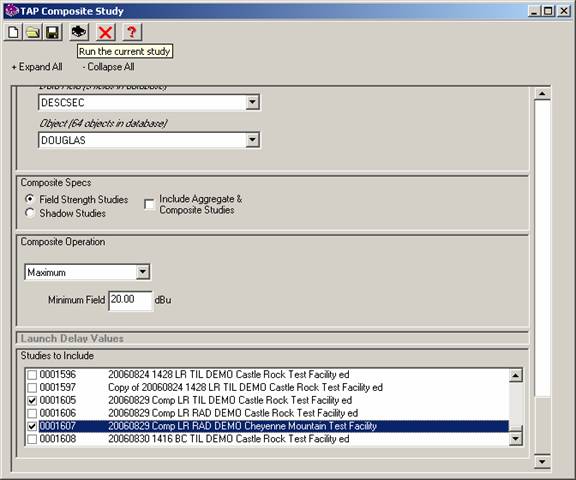
Composite Specs
Select the option of Field Strength Studies or Shadow Studies. The Composite Study can be used with Shadow studies to determine the best line of sight to each location from multiple transmitter sites. For this example, select Field Strength Studies:
If you want to combine the results of other Aggregate or Composite studies in this Composite study, check the box on the form. For this example, leave the box empty.
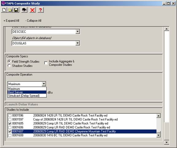
Composite Operation
Select the operation to use with the points from the different coverage studies. The Maximum option simply selects the highest of the field strength (or shadow ratio) levels.
For this example, select the Maximum option:
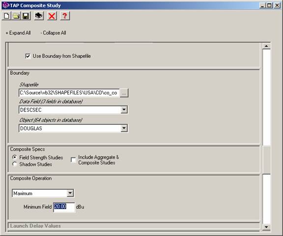
Enter the minimum field strength level for the example, 20dBu, the same value shown on the map with the individual studies at the beginning of this article.
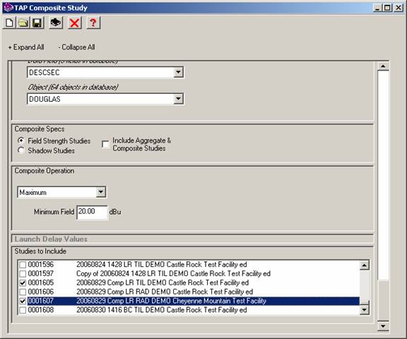
Tasks to Include
The list near the bottom of the form displays Tile and Radial studies computed in TAP. The list will be refreshed if you change the "Field or Shadow" option, or the "Include Aggregate…" option.
Click the checkbox at the left of the lines for each study you want to include.
The two studies shown at the beginning of this article are selected:
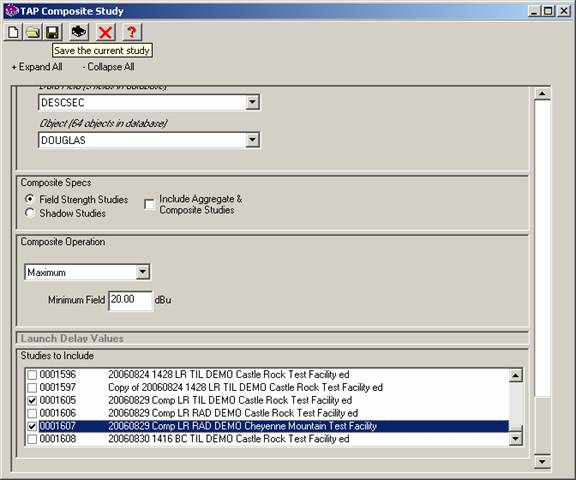
With all the settings made, click the Save button on the toolbar near the top of the form to save the settings.
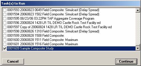
When you are ready to run the study, click the Run button on the toolbar near the top of the form.
The Tasks to Run list will be displayed. Any studies you have edited and saved during this session will be checked in the list. You can add or remove checks to determine which studies will be run during this calculation.
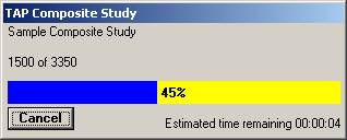
The study will take several seconds to set up, then a progress form will be displayed.
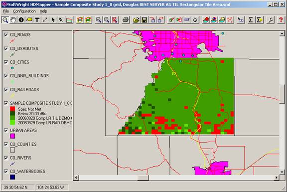
When the study is completed, the results will be displayed in HDMapper (if the AutoDraw box was checked when you set up the study).
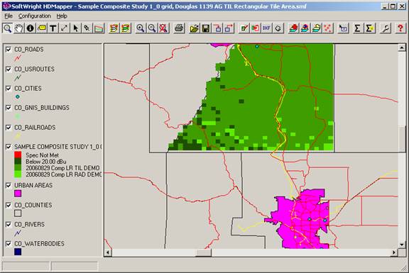
The legend shows the results of the composite calculation:
□ Spec Not Met indicates the requirements of the Composite Study were not met. This value is usually not of significance in Maximum studies (like this one). However, if there are points on the composite grid that have no points from the original studies, those points will be shown as Spec Not Met, since no calculation could be performed. Other types of Composite Studies, such as “Best Server” or “Simulcast Delay Spread” have other criteria that are required for the composite points to be computed. In these cases, the Spec Not Met designation indicates those specifications were not achieved at the points.
□ Below 20 dBu indicates that none of the points in the source coverage studies were above the minimum (20dBu) specified for this study.
□ The remaining entries show which of the source studies was used for the composite point. In this example there were two source studies, so there are two additional legend entries.
You can change the Layer settings to make the Spec Not Met and Below 20dBu points transparent, showing only the points served by one or the other of the source sites:
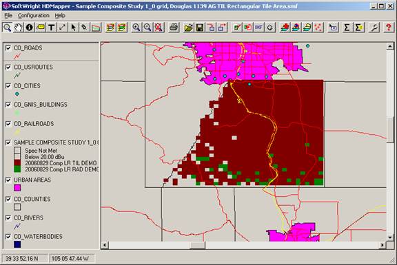
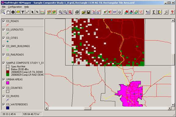
As a comparison, if you ran the same study with the north, south, east and west limits but not using the Douglas County shapefile object, the results would show the entire rectangular area bounding the county:
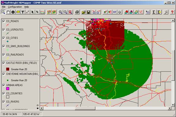
You can also compare these results with the original map showing the two coverages drawn separately, not considering the composite calculation:
Or, changing the layer order of the two independent studies:
The Composite Study enables you to see the actual coverage from each site more clearly.
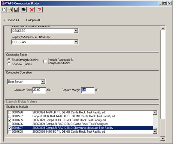
Best Server Study
The Maximum Composite Study shows the maximum value at each location from the two source sites. But you may also want to include other information. For example, the Best Server study finds the highest signal level at each location (just as the Maximum study) but also checks for a Capture Margin, the difference between the highest signal at a location and the other signals.
For example, if a manufacturer’s specification states that a receiver requires at least 8dB of isolation from other signals to operate you can run a Best Server study and include an 8dB Capture Margin. That means that even at locations where one of the source sites provides adequate signal, if any other site also provides a signal within 8dB of that highest value, the location is marked as “Spec not met”, since the Capture Margin specification was not achieved.
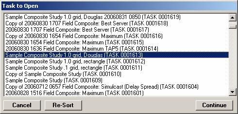
As an illustration, we can open the Composite study we ran for Douglas County with the Open button on the toolbar near the top of the form:
From the list of Composite Studies that is displayed, select the one to open:
When the Task is loaded, the program will prompt you to create a new task.
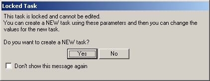
Once a Task in TAP has been run, the Task is “Locked” to prevent confusion if settings are changed, making the Task parameters inconsistent with the Task results. Creating a new Task will keep all of the same settings and assign a new Task ID. Then you can make changes to the settings and run the new Task.
A new Task is created with the same settings. The Task Description is the same as the original, with the prefix “Copy of …” added:
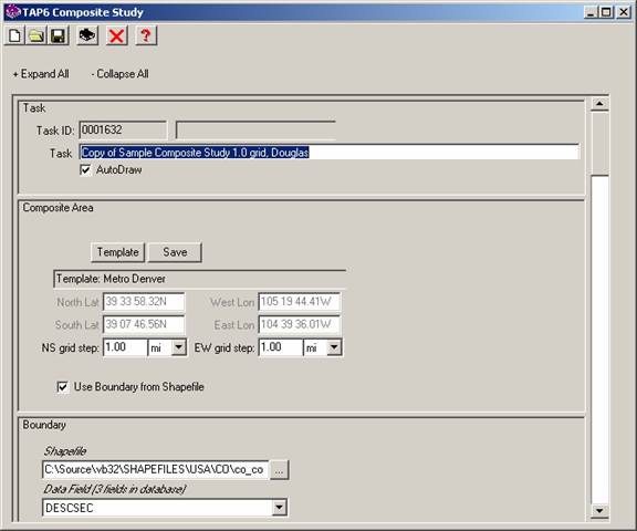
Scroll to the Composite Operation section and select Best Server from the list:
When the Best Server option is selected, the Capture Margin input box is displayed. Enter the desired value (8dB in this example):
It is always a good practice to make the Task Description as specific as possible for finding the information later:
When you save and run the Best Server study for the same area, the results are displayed in HDMapper:
Note in this case there are numerous locations where the signals from the two sites do not meet the Capture Margin requirements.
|
|
Copyright 2006 by SoftWright LLC