Shadow Levels in TAP6
Q: When I run a shadowing study, how do I determine areas of clear line of sight, shadowing, etc.?
A: The shadow study in TAP computes a "shadow ratio" for every point in the study (along radials or in a tile area). The shadow ratio is the lowest value along the path of the ratio between clearance at each point along the path and the first Fresnel zone at the specified operating frequency. The shadow ratio represents the worst case obstruction along the path.
The clearance at each point is defined as the distance between the elevation of the topography at that point (adjusted for earth curvature) and the elevation of the line of sight path at the same location. A positive value indicates that the line of sight path is above the terrain at that point. A zero or negative value indicates that the terrain is higher and the line of sight is blocked. A negative clearance value will also result in a negative shadow ratio.
The shadow ratio defines the "worst case" shadowing for the path. For example, it only takes one point to block the line of sight along a path. If several points of the terrain block the line of sight, the shadow ratio for the path will be based on the point with the worst "clearance-to-Fresnel" ratio. This gives some quantitative information about blocked paths: the lower the negative value, the worse the blockage is. In the same way, positive shadow ratios indicate the relative amount of clearance on a clear line of sight path.
The values for traditional shadow studies can be based on the shadow ratios.
· Any path with a zero or negative ratio (i.e., less than or equal to zero) is blocked.
· Any path with a positive ratio (i.e., greater than zero) has clear line of sight.
· Grazing paths can be defined using half the first Fresnel zone, so any path with a ratio less than .5 (but greater than zero) can be considered grazing. (Some engineers prefer to use .6 of the first Fresnel zone.)
In HDMapper you have the opportunity to set shadow levels to plot, similar to field strength threshold levels, with different colors and/or fill patterns for different levels.
For example, suppose you have a shadow study you have run in HDCoverage and plotted in HDMapper:
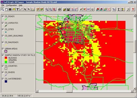
This map shows the three default shadow ratio levels.
It might be useful to show areas where there is only minimal line of sight obstruction. Any shadow ratio less than zero indicates a blocked line of sight, but small negative values are less obstructed than higher negative values. As an example, we can add another level showing areas of shadow ratio between 0 and -0.1 would indicate areas of borderline blocked paths.
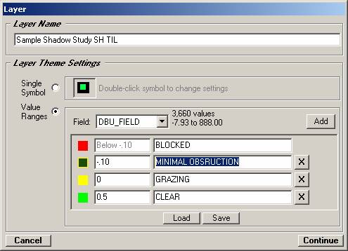
To add another shadow ratio to plot, double-click the “Sample Shadow Study” legend entry. The Layer form is displayed:
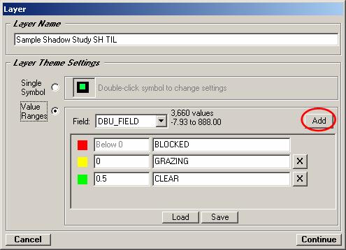
Click the Add button to add another level:
A new level is added at the end of the list. The initial value (by default) is halfway between the highest level and the maximum value in the file. This value is usually not of any practical significance and is usually changed before plotting.
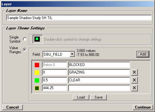
For this example, change the default level value to the
new desired shadow ratio to plot,
–0.1
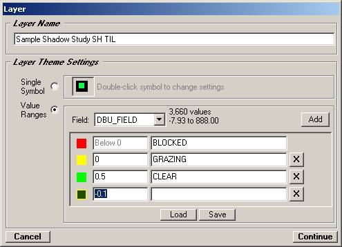
When you move the mouse cursor out of the text area, the program accepts the value, and the list is automatically sorted in ascending order. Enter a description to include in the legend for this level:
Click the Continue button to accept the present settings. The new level is added to the shadow plot:
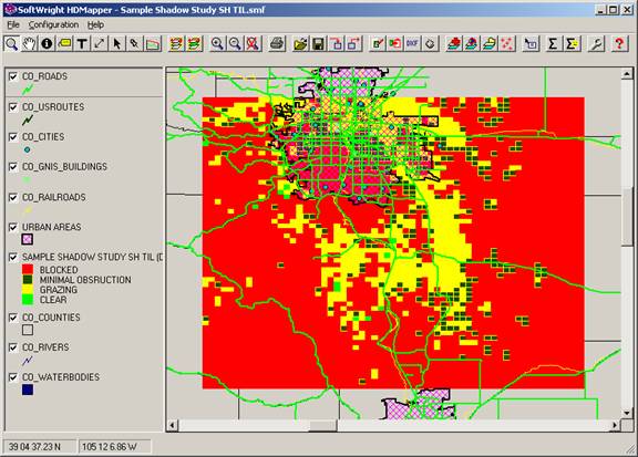
You can set and plot other levels of shadow ratios that are useful in your application.
|
|
Copyright 2007 by SoftWright LLC