TAP6 Coverage with Directional Antenna
Q: Why doesn’t my coverage calculation look like the shape of the directional antenna I used?
A: Several factors affect the computed coverage information in addition to the antenna pattern.
For example, consider two coverage studies, one computed as an omni-directional coverage, with no antenna pattern specified, and one with a specific antenna. For the two studies, all other factors were exactly the same.
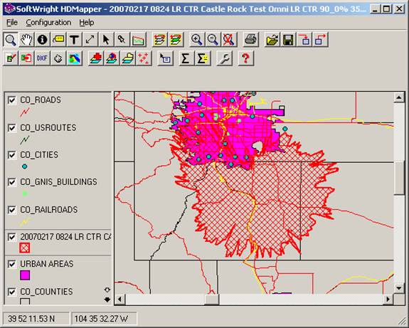
First, the coverage from the omni study is shown:
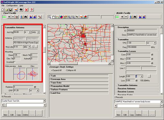
The same study was run again with the addition of a directional antenna pattern:
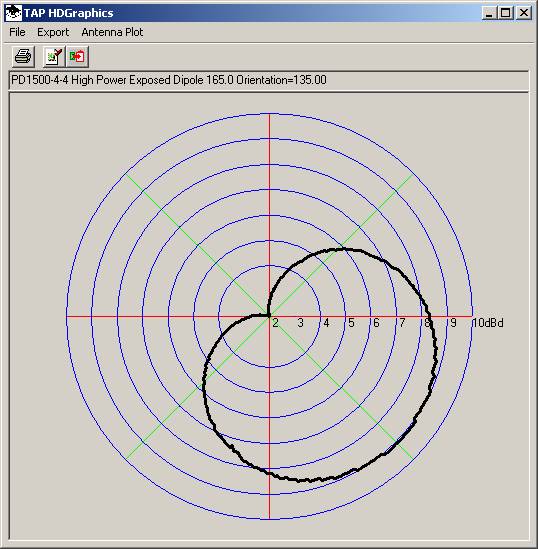
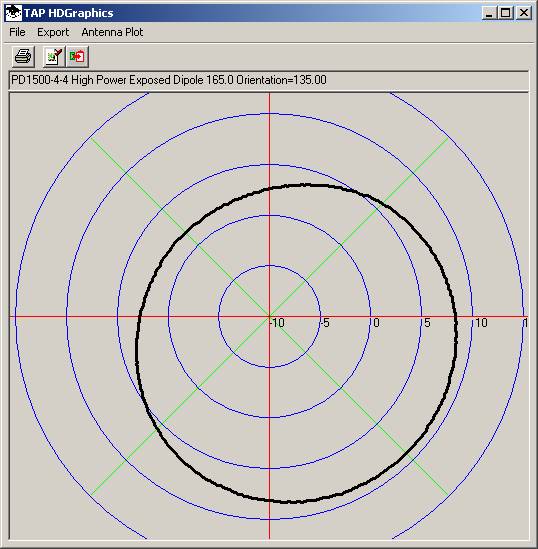
The pattern used is plotted below, with the orientation of 135 degrees used in the study with the antenna included:
The computed coverage using the antenna is shown below:
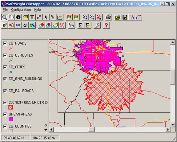
The resulting coverage plot clearly shows the effect of the antenna (to focus the radiated power to the southeast). However, the shape of the coverage shown by the field threshold points and the contour (the 35.8dBu, 90% contour computed from the radial field calculations) does not reflect the exact shape of the antenna pattern.
If you include a directional antenna pattern in the HDCoverage Setup and keep the Effective Radiated Power (ERP) the same as the omni calculation, the major lobe of the antenna will have the same power (and the same coverage) as the omni calculation. This is demonstrated to the southeast in the coverages shown. Since the directional coverage was computed with the antenna orientation at 135 degree azimuth, we would expect the coverage to look the same in that direction.
Other directions from the transmitter site, where the antenna gain is reduced from the major lobe radiation, will show reduced signal levels. Again, this is shown in the areas to the north and northwest of the transmitter site, where the signal levels are significantly below those shown on the plot of the omni calculation.
A couple of other considerations:
(1) When you add the antenna pattern, if the antenna in the TAP library includes an elevation (vertical plane) pattern, the directionality in the vertical plane is also considered, so the coverage will not look exactly like the plot of the antenna pattern.
(2) The computed field strength depends on a number of other factors besides the transmitted power from the antenna to each computed receiving point, such as the intervening terrain, the propagation model used, etc. In many cases, these other factors, such as the terrain, can have a greater impact than relatively small differences in power on different azimuths. This is especially true with antennas that do not have large differences in gain between the major lobe and antenna nulls. The coverage will not follow the exact shape of the pattern. In the example above, the coverage in the minimum radiation portion of the pattern was over water, so even the reduced power in that direction did not have a dramatic effect on the coverage when shown as a contour.
(3) Most antenna plots are drawn using units of dBd or dBi. Changing the scale on the plots can help to identify nulls in the pattern or other details. But changing the scale on the plot can also give a distorted image of what to expect from the antenna pattern. Again, this would cause the plot of the coverage from the antenna to look quite different from the plot of the antenna pattern at a particular dB scale range.
Consider the directional antenna pattern used in this example. When plotted with the default polar plot range (+2dB to +10dB), the pattern appears as shown below:
However, changing the scale range minimum (the center of the polar plot) to –10dBd results in a different appearance for the plot of the same antenna:
These differences in the appearance of a plot for the same antenna clearly illustrate that the shape of the antenna pattern does not necessarily indicate the shape of the resulting coverage computed using the antenna.
|
|
|
Copyright 2007 by SoftWright LLC