TSB-88 Coverage Analysis Assessment

    Q: Using TAP 6, how do I run a TSB-88 based map? 

    A:  The TIA/EIA Telecommunications Systems Bulletin (TSB) – 88B titled, Wireless Communications Systems – Performance in Noise and Interference – Limited Situations – Recommended Methods for Technology – Independent Modeling, Simulation, and Verification, provides recommendations for predicting land mobile radio coverage and for verification of the coverage as the title suggests.  These recommendations are often specified as requirements that must be verified by a standard way of testing the radio coverage.  Because TSB-88 requirements are increasingly being specified, it’s important for TAP users to understand how to generate coverage maps that will meet the TSB-88 recommendations and that will hold up to review and verification by consultants, customers and peers.  TSB-88’s recommendations/requirements are based upon input from major radio manufacturers and from consultants within the land mobile industry.     

 

Because TAP 6 has been designed for maximum flexibility, it’s possible to generate coverage plots that follow the TSB recommendations/requirements.  The following procedures for generating TSB-88 based maps using TAP 6 have not been tested against the TSB-88 coverage testing recommendations/requirements at this time.  It’s important that the TAP user calibrate their TSB-88 based coverage plots to implemented systems to ensure a successful coverage prediction and coverage test.  This calibration is necessary whether generating “regular” coverage plots or TSB-88 based coverage plots.  Softwright encourages real system feedback and calibration values and will update these procedures and settings accordingly.

 

TSB-88 Terminology

 

The following defines some of the key TSB-88 concepts or terms.  These definitions come from public Coverage Acceptance Test Plans (CATP), TSB-88 and from TIA TR8 Working Group 8.8.  TSB-88 is based upon TIA TR8 Working Group 8.8’s report and it can be found at http://www.antd.nist.gov/wctg/manet/docs/TIAWG88_20.pdf . 

 

It’s important to learn these terms and to learn how they apply to the TAP 6 application if running TSB-88 based maps:

 

Coverage Area or Service Area:

The coverage area is the geographical region where communications will be provided which meets or exceeds the specified Channel Performance Criterion at the specified reliability for the specified equipment configuration.  Typically radio systems are designed to maximize the coverage area within the customer’s service area (users’ operational area, jurisdictional boundaries, etc.) {TSB-88, clause 4.1 [3]} 

 

Channel Performance Criterion (CPC):

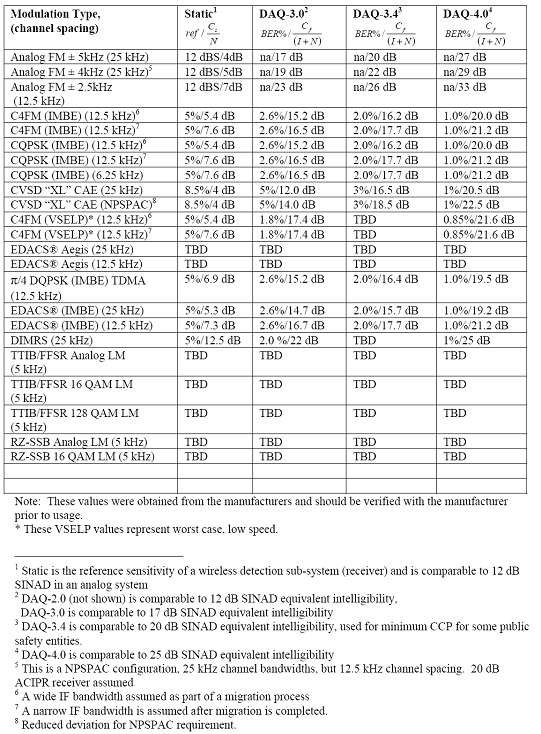
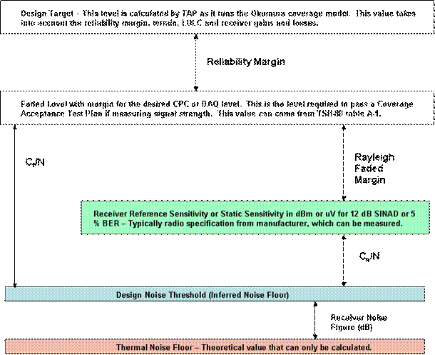
The CPC is the specified minimum design performance level in a faded channel. {TSB-88, clause 4.2 [3]}  For most public safety systems, the CPC is a Delivered Audio Quality of 3 (or DAQ-3); the DAQ definitions are provided in Table 1. {TSB-88, Annex A, Table 1 [3]}.  Given the static reference sensitivity of a receiver, the faded performance threshold for the specified CPC is determined by using the projected CPC requirements for different DAQs listed in TSB-88, Annex A, Table 5.  The CATP pass/fail criterion for each test location is the faded performance threshold, plus any adjustments for antenna performance and in-building losses.  {TSB-88, subclause 4.5.1, Figure 2 [3]}. 

 

Table 1 – Delivered Audio Quality Definitions

 

Reliability:

The reliability is the percent of locations within the coverage area, which meet or exceed the specified CPC.  TSB-88 based coverage maps indicate the area for a given radio system that is predicted to provide the specified reliability (typically 95%) and meet or exceeding the CPC.  {TSB-88, subclause 4.4.1; not regulatory contour reliability [3]}

 

TSB-88 talks about two different kinds of reliability, contour and area.  Contour reliability (not to be confused with regulatory type contours based upon a radials) will show all points/grids that meet or exceed the CPC.  Area reliability will not only show all points/grids that meet or exceed the CPC, but it will also show some grids that don’t meet the CPC such that all grids in the service area meet or exceed the reliability. 

 

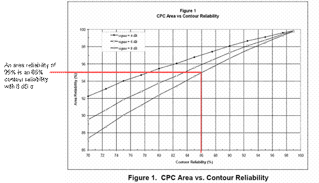
The following figure 1 shows a conversion chart between contour reliability and Area reliability for a constant power loss exponent of 3.5, and for a perfectly flat sphere and for three different values of σ.  The chart comes from TIA TR8 Working Group 8.8 [1] and it’s based upon equations which can be found from Ruedink [2]   

 

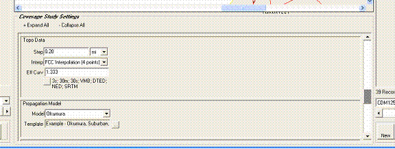
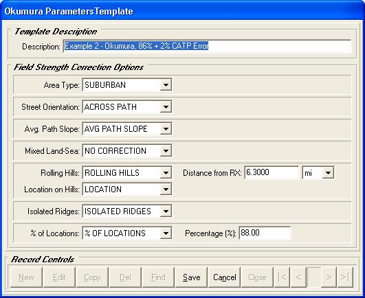
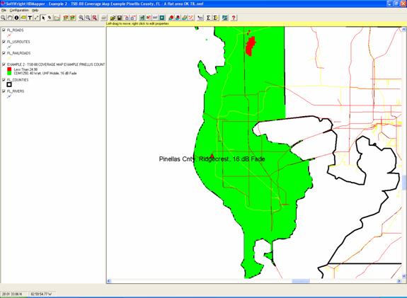
Tap 6 currently predicts a contour reliability.  Area reliability is typically easier for an end user to understand and when compared with a contour map will show the greatest coverage.  For example, based upon figure 1, one could show a TAP 6 contour map that shows all grids predicted to have sufficient signal strength to provide a DAQ audio level of 3.0 at 95% reliability.  The fringe areas of this map reflect a contour where the reliability of each grid contained in the contour will achieve the DAQ of 3.0.  Based upon figure 1 this map would reflect an area reliability of 98% to 97%.  Again based upon the chart to achieve an area reliability of 95% then the Contour reliability or signal strength shown would be considerably less at 86% for 8 dB σ. 

 

 

 

The best way to demonstrate a coverage plot and generation of a TSB-88 map with TAP 6 is to use the following example. 

 

Example coverage requirement:

Predict coverage for Pinellas County, FL that will give Delivered Audio Quality (DAQ) value of 3.0 for 95% of the time throughout 95% of the county using UHF Narrow Band FM modulation and using the latest version of TSB-88 as coverage requirements.    

 

Mobile Radio:  Motorola CDM 1250, with 3 dB gain antenna at the 9 foot level and 40 Watts of transmitter power. 

 

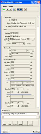
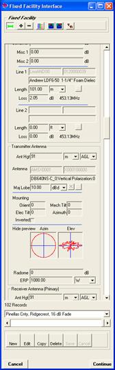
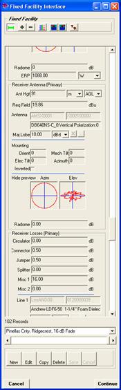
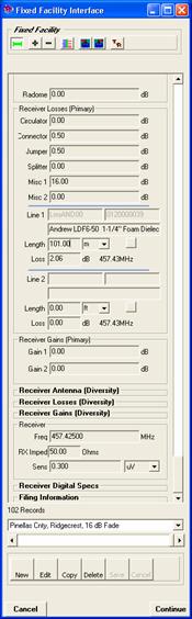
Fixed Facility: Called RIDGECREST will use a Motorola MTR2000 station with 10 dB of gain, an OMNI antenna at 91 meter level and an ERP of 1088 Watts:

 

Fixed Facilty Name: RIDGECREST 

Lat (NAD83): 27-53-06.1 N Long (NAD83): 082-48-38.4 W

Frequency: 453.125 MHz 250 Emission Designator: 16K0F1D => Narrow Band operation
ERP: 1088 Watts  Antenna Height:  91.0 Meters  

 

Given:

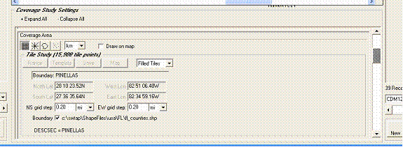
• Service area are the boarders for Pinellas County (TAP 6 has the shape file for many Counties and Cities in the US)
• This will be an area map and the area reliability is 95%
• Channel Performance Criteria is Delivered Audio Quality (DAQ) level of 3.0 or from table 1, “Speech understandable with slight effort.  Occasional repetition required due to Noise/Distortion”
• Frequency for base station TX = 453.125 MHz, RX = 458.125 MHz
• Site information
• Radio information
• Base station information
• TSB-88 information   

 

Procedures:

1. For the fixed facility that is using the MTR2000 repeater, vendor specific information is required.  This information is typically found at the vendor’s website.  In this case the MTR2000 repeater’s specifications were found at: http://www.motorola.com/governmentandenterprise/contentdir/en_US/Files/ProductInformation/mtr_2000_800_900_catsheet.pdf  .  Likewise specific information is required for the mobile facility.  In this case the CDM1250’s specifications were found at:  http://www.motorola.com/governmentandenterprise/contentdir/en_US/NonXMLDocs/MD-CDM1250-01c_cdm1250_specs.pdf .
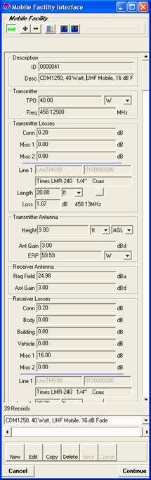
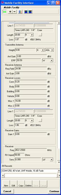
2. Using the fixed facility repeater information and the other site information create the fixed facility.  Using the mobile radio information, create the mobile facility.  The following screen shots show how the fixed facility and mobile facility was created for this example using TAP version 6.

 

Fixed Facility Screen Shots:

 

 

 

 

 

 

 

 

Mobile Facility Screen Shots:

 

 

 

 

 

 

Notice that all settings are similar to other FAQ’s for running a TAP 6 map, except for the additional loss added to the repeater and the mobile radio receivers.  This additional loss of 16 dB under Misc. 1 is the required/recommended margin to achieve the given CPC.  The margin comes from table 2 which comes from [2] TIA TR8 Working Group 8.8’s report’s table 5 and which comes from table A-1 in Annex-A of TSB-88 [3].  The following diagram explains how the gains and losses add up for the final dBu value in TAP 6.

 

Table 2 – Projected CPC Requirements for Different DAQs

 

 

Figure 2 – Fadded Sensitivity and Design Target Budget

 

For this example, both the fixed facility and the mobile radio will use analog FM Narrow Band operation.  From table 2 the 12 dB reference static Cs/N for this configuration is 7 dB.  The value for a DAQ 3.0 is 23 dB.  The difference (23 dB – 7 dB = 16 dB) of 16 dB is the additional loss that we must add to each facilities receiver to ensure that we will meet the DAQ 3.0 requirement.  In this example, the loss has been added to Miscellaneous Loss # 1 field, but it could be added in Miscellaneous Loss # 2 or rolled in with line loss or taken away from receiver sensitivity manually.  The author finds it easiest to track if it is placed in one of the miscellaneous fields.   

 

3. Now it’s time to set up the area coverage study.  This part is very similar to other FAQ’s for TAP 6.  The only exception is that TSB-88 recommends using the Okumura prediction model {TSB-88, clause 6 [3]} and because we are generating an area reliability coverage prediction, we can lower our Okumura reliability settings to reflect what the contour reliability should be.  Per figure 1 one can set the reliability setting to 86% to achieve an area reliability of 95%.  Note that this is a first order approximation which is likely valid for a flat area such as Florida.  For other areas the terrain should be considered and future utilities or tools may be made available to assist in this endeavor.     

 

TSB-88 not only recommends on how to predict coverage, but it also recommends on how to test coverage.  TSB-88 allows for a Coverage Acceptance Test margin in estimating the number of grids to test using the Estimate of Proportions {TSB-88 subclause 7.1 [3]}.  For this example, a CATP error margin of 2% will be used.  Thus the value for Okumura reliability will be 88%.  The following screen shots show the values used for this example. 

 

 

 

 

 

 

 

 

 

 

4. Run the prediction.  For this example the following talk – out prediction was generated. 

 

By right clicking on the mobile radio and selecting coverage statistics on the context menu, the following coverage statistics are displayed: 

 

Example 2 - TSB-88 Coverage Map Example Pinellis County, FL - A flat area OK TIL

 

Coverage Statistics

 

C:\SWTAP\MAPPING\MAP FILES\Example 2 - TSB-88 Coverage Map Example Pinellis County, FL - A flat area OK TIL\Example 2 - TSB-88 Coverage Map Example Pinellis County, FL - A flat area OK TIL.SHP

 

 0.76%

            BELOW 24.98dBu (66 of 8722)

 

CDM1250, 40 Watt, UHF Mobile, 16 dB Fade 99.24%

            24.98dBu (8656 of 8722)

 

99.2% of all tiles exceed the 88% reliability.  Thus this map is predicting that the coverage requirement listed above is being met:

 

“Predict coverage for Pinellas County, FL that will give Delivered Audio Quality (DAQ) value of 3.0 for 95% of the time throughout 95% of the county using UHF Narrow Band FM modulation and using the latest version of TSB-88 as coverage requirements.”   

 

References

 

[1] Telecommunications Industry Association, A Report on Technology Independent Methodology for the Modeling, Simulation and Empirical Verification of Wireless Communications System Performance in Noise and Interference Limited Systems Operating on Frequencies Between 30 and 1500 MHz, TIA TR8 Working Group 8.8, 20 May 1997,  http://www.antd.nist.gov/wctg/manet/docs/TIAWG88_20.pdf

 

[2] Ruedink, Douglas O., “Chapter 2: Large-Scale Variations of the Average Signal”, in: W.C. Jakes ed., Microwave Mobile Communications, New York: Wiley, 1974, Reprinted by IEEE Press, 1993, ISBN 0-471-21824-X

 

[3] TIA/EIA Telecommunications Systems Bulletin (TSB), Wireless Communications Systems – Performance in Noise and Interference – Limited Situations – Recommended Methods for technology – Independent Modeling, simulation, and Verification, TSB88-A, June 1999

 

 Our thanks to Orbital Sciences Corporation, Columbia, MD,  and Mr. Robert Bridenstine for making this information available.