Introduction
The Bullington field strength contour and threshold programs are accessed in the Coverage options of the TAP main menu. These programs use data extracted from the topographic data to compute terrain shadowing effects on free-space field strength values.
The method of computing terrain attenuation is described in "Radio Propagation for Vehicular Communications," by Kenneth Bullington (IEEE Transactions on Vehicular Technology, vol. VT-26, no. 4, November 1977). Obstruction losses are computed by the method associated with Figure 10 of that paper ("Transmission loss versus clearance"). (This method is used by the National Bureau of Standards for computing field strengths in the protected Table Mountain quiet zone near Boulder, Colorado. Extensive field strength measurements demonstrate the accuracy of the Bullington method.) Both programs use the same method of computing free-space field and terrain attenuation.
Obstruction Selection
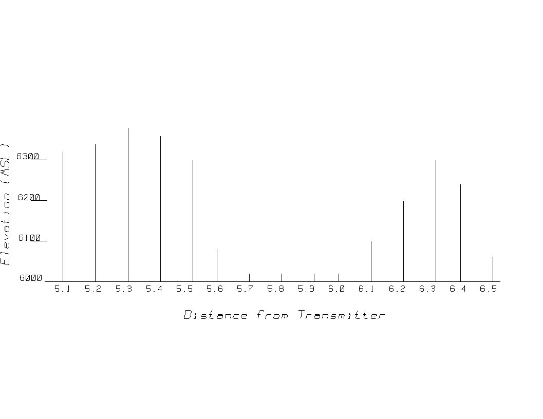
After terrain elevations have been retrieved for a particular Project, the elevation data file consists of numerous discrete elevation points as illustrated below:
When a the path is analyzed for propagation losses, the line of sight from the transmitting antenna to the receiving antenna, and the associated Fresnel zone are computed. Attenuation from terrain obstructions is predicted whenever the obstructions penetrate half of the first Fresnel zone, as illustrated below:
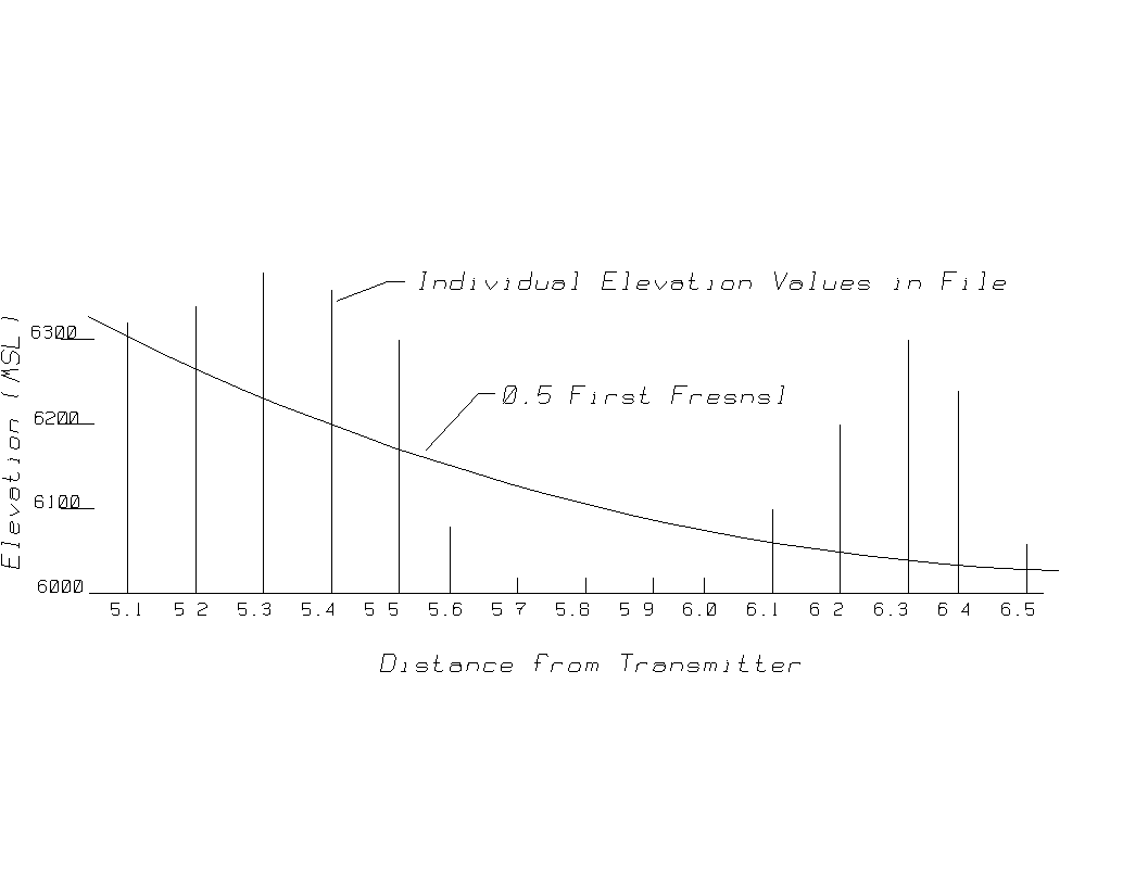
If each of the data points in the elevation file is treated as an obstruction, the computed attenuation will usually be exaggerated. For example, the obstructions at 5.3 miles and 6.3 miles on the path shown would be reasonable points to use in computing the. If all of the points that penetrate the Fresnel zone are included, the computed attenuation will be higher, possibly producing erroneous results.
For example, the computed loss values around the peaks at 5.3 miles and 6.3 miles might indicate the following:
Distance Elevation Path Loss
5.1 mi 6320 -0.5 dB
5.2 mi 6340 -1.2 dB
5.3 mi 6370 -3.1 dB
5.4 mi 6350 -3.0 dB
5.5 mi 6300 -0.2 dB
6.0 mi 6000 -0.3 dB
6.1 mi 6100 -1.0 dB
6.2 mi 6200 -2.5 dB
6.3 mi 6300 -3.0 dB
6.4 mi 6150 -2.0 dB
6.5 mi 6050 -0.8 dB
-------
-17.6 dB Total loss
If the program treats each data point independently as a knife edge peak, the resulting loss prediction (17.6 dB) will be inaccurate. Normally, careful engineering analysis is necessary to determine the realistic losses expected on such a path.
In order to automate the process of selecting which obstruction points to include in the calculations, the TAP field strength programs provide two methods: one method is based on a minimum distance between obstructions; the other is based on points of inflection in computed loss values.
Minimum distance between obstructions
The first method of selecting obstructions is based on a user-specified minimum distance between obstructions. A single obstruction in a path may be represented by several adjacent data points in the elevation file. In order to prevent all of the points from being used, a "minimum distance between obstructions" can be specified. (The user-specified minimum distance is inclusive. For example, if a minimum distance of one mile is specified, obstructions that are separated by a distance greater than or equal to one mile will be considered as separate obstructions
This method uses the following process:
The loss is computed for every data point in the elevation file.
All of the loss values for the path are sorted in order of descending loss values.
The greatest loss value (which is first in the sorted order) is included in the loss calculation for the path.
The successive loss values (in the sorted order) are ignored until a loss value is found which is associated with an obstruction that is at least the "minimum distance" from the obstruction associated with the first loss value.
This process is continued, considering all of the computed loss values in the sorted order. In every case, loss values that are less than the minimum distance from any other selected loss value are ignored.
This method tends to isolate the peaks along a path.
For example, assume a minimum distance between obstructions of 1.0 miles is specified. Applying this method to the sample elevation values results in the following sorted loss values:
Distance Elevation Path Loss Include?
5.3 mi 6370 -3.1 dB Yes
5.4 mi 6350 -3.0 dB No
6.3 mi 6300 -3.0 dB Yes
6.2 mi 6200 -2.5 dB No
6.4 mi 6150 -2.0 dB No
5.2 mi 6340 -1.2 dB No
6.1 mi 6100 -1.0 dB No
6.5 mi 6050 -0.8 dB No
5.1 mi 6320 -0.5 dB No
6.0 mi 6000 -0.3 dB No
5.5 mi 6300 -0.2 dB No
As this tabulation illustrates, only the loss values computed for the obstructions at 5.3 miles and 6.3 miles would be included in the loss calculations for this path, resulting in a cumulative loss prediction of 6.1 dB. None of the other obstructions listed meets the 1.0 mile minimum distance. Especially note the 3.0 dB loss from the obstruction at 5.4 miles. Because this obstruction does not meet the minimum distance, the loss is ignored.
The minimum distance between obstructions is user-selectable, and different values will result in different results. Typical minimum distance values are in the range of one to two miles. Extremely small minimum distance values (e.g., 0.1 - 0.2 miles) will usually result in an overestimate of loss values.
Critical paths should still be examined in detail by plotting the path profile and selecting the obstructions using careful engineering judgment. Then use the single field" program to compute the losses on the path individually.
Loss Value Inflection
The second method considers points of inflection in the computed loss values along the path. The point of inflection is the point where increasing attenuation begins to decrease, i.e., a peak in the attenuation
This method uses the following process:
The attenuation caused by each point on the path is computed.
The attenuation for each point is compared with the attenuation from the previous point.
A point of inflection is found when both the point before and the point after result in lower attenuation than the current point. The attenuation from current point is then included in the loss calculation for the path.
Distance Elevation Path Loss Increase/Decrease
5.1 mi 6320 -0.5 dB Increase
5.2 mi 6340 -1.2 dB Increase
5.3 mi 6370 -3.1 dB Increase
5.4 mi 6350 -3.0 dB Decrease
5.5 mi 6300 -0.2 dB Decrease
6.0 mi 6000 -0.3 dB Increase
6.1 mi 6100 -1.0 dB Increase
6.2 mi 6200 -2.5 dB Increase
6.3 mi 6300 -3.0 dB Increase
6.4 mi 6150 -2.0 dB Decrease
6.5 mi 6050 -0.8 dB Decrease
This tabulation shows the inflection method applied to the sample elevation values shown above. In this example, the points of inflection in the loss calculations (where increasing values begin to decrease) occur at 5.3 miles and 6.3 miles.
In general, the minimum distance method will prove more useful if the terrain is relatively flat. This is because the inflection method will interpret very small changes in loss calculations over flat terrain as inflection points, adding too many points into the attenuation calculations.
The inflection method will prove more useful in mountainous or hilly terrain. The definitive increases and decreases in computed loss values allow the inflection method to isolate terrain peaks that should be included in the attenuation calculations, independent of the distance between the peaks.
Obstacle Peak Method
The Obstacle Peak method is described in a separate article.
Figure 12 Method
The Figure 12 method is described in a separate article.
Note that all selection methods are approximations used to automate the process, allowing rapid calculations of large numbers of field strength values. Critical paths should be examined carefully to ensure that loss calculations are based on good engineering judgment.
Field Strength Calculation
The program computes the field at each point specified by the user by the following process:
Compute the free-space field at the target point (given the effective radiated transmitter power and directional antenna relative field information).
Determine the elevation of the target point from the terrain data. (If the target point is beyond the data in the file for the radial, the elevation of the last point on the radial is used. When this occurs, a notation will be included on the printed output. For more reliable predictions, elevation data should be extracted beyond the expected contour distance, and the Bullington field program executed again.)
For each elevation data point on the radial between the transmitter site and the target point:
Compute the elevation of the line-of-sight path from the transmit center of radiation to the target point (adjusted for the receiver height above ground specified).
Compute the elevation of one-half of the first Fresnel zone for the line-of-sight path.
Correct the elevation of the terrain data point for earth curvature, considering the path length from the transmitter site to the target point.
If the terrain point penetrates the Fresnel zone (i.e., the corrected terrain elevation is higher than the computed Fresnel zone elevation), compute shadowing loss resulting from this elevation data point.
After each elevation data point on the path has been evaluated, determine the net received field at the target point, including loss values for the minimum distance or inflection method described above.
This process is repeated for every specified "target" point. Loss calculations for the terrain closest to the transmit site are computed many time
|
|
I'm interested! Please click here to jump to an online form which helps us better understand your needs. Then we will be able to respond to your request with information that is most useful to you. |
|
|
Copyright 2000 by SoftWright LLC